
 Open Access Article
 This Open Access Article is licensed under a
 Creative Commons Attribution 3.0 Unported Licence
A microfluidic chip integrated with droplet generation, pairing, trapping, merging, mixing and releasing†
Xiaoming Chen and
Carolyn L. Ren *
*
Department of Mechanical and Mechatronics Engineering, University of Waterloo, 200 University Ave W., Waterloo, ON, Canada N2L 3G1. E-mail: c3ren@uwaterloo.ca; Fax: +519-888-4567; Tel: +519-888-4567 ext. 33030
First published on 16th March 2017
Abstract
Developing a microfluidic chip with multiple functions is highly demanded for practical applications, such as chemical analysis, diagnostics, particles synthesis and drug screening. This work demonstrates a microfluidic chip integrated with a series of functions including droplet generation, pairing, trapping, merging, mixing and releasing, and controlled entirely by liquid flow involving no electrodes, magnets or any other moving parts. This chip design is capable of trapping and merging droplets with different content on demand allowing the precise control of reaction time and eliminates the need for droplet synchronization of frequency, spacing or velocity. A compact model is developed to establish a set of design criterion. Experiments demonstrate that fast mixing in the merged droplets can be realized within several seconds benefiting from the flow fluctuation induced by droplets coming or leaving the trapping region. Additionally, it allows a concentration gradient of a reagent to be established. Finally, this design is applied to screen drug compounds that inhibit the tau-peptide aggregation, a phenomenon related to neurodegenerative disorders.
1 Introduction
Droplet microfluidics has attracted ever-increasing attention from both academy and industry due to its complex transport phenomena and broad potential applications in chemical analysis,1 diagnostics,2 particle synthesis,3 and drug discovery.4,5 Droplet microfluidic technology manipulates femto-litre to nano-litre volumes of reagents in droplets that are fully compartmentalized by the other immiscible fluid, and hence has numerous advantages over single-phase microfluidics such as high throughput, low sample consumption, rapid mixing and no cross-contamination with perfect wetting conditions.6 Despite the success in developing droplet microfluidic devices for various applications and gaining fundamental understanding of complex droplet transport phenomena, many challenges remain to make droplet microfluidics an enabling technology for high throughput combinatorial testing. Among the many challenges such as demand for ideal surfactants for different fluid pairs, lack of physical models for design and operation, and still expensive mass production of chips with perfect wetting properties; robust functionalities for droplet manipulation is one of the hurdles.7 A typical chemical or biomedical reaction requires multiple steps of droplet manipulation, which has driven numerous studies on droplet generation,8–11 transport,12–14 pairing,15 trapping,16–19 merging,20–23 mixing,24 and sorting,25–27 either actively or passively. Developing each individual function with robust performance is very challenging, let alone the integration of multiple functions which is highly demanded for practical applications.Several groups have reported droplet microfluidic systems integrated with multiple functionalities and successfully applied them for protein crystallization evaluation,28 apoptosis analysis of cells29 and nanoparticle synthesis.30,31 One of the common challenges for these reported designs is the difficulty in controlling the reaction start time because two different reagents already contact with each other before droplet generation. Although reaction might only occur slightly at the interface, it is not ideal and might vary between different reactions. An improved strategy was reported later to inject a small amount of reagent into a passing droplet,32,33 which is prone to cross contamination though.34 The use of integrated pillars for droplet merging,23 where a second droplet stream containing the new reagent is merged with the original droplet stream could also control the reaction start time, but requires synchronization between the generation of the two streams of droplets which is very sensitive to operational uncertainties such as pressure fluctuations.
To address the above concerns and also meet the needs of many practical applications such as drug screening and decorating nanoparticles for DNA sensing which require a concentration gradient of a particular reagent to be established for screening, a droplet microfluidic system should be capable of generating droplets with two or more different sample fluids, trapping and merging them on demand in order to control the reaction starting time or observe particle–particle interaction. This motivation prompts the work reported here. In this work, we demonstrate a microfluidic channel network design that is able to generate, pair, trap, merge, mix and release two streams of droplet with two different types of reagents. This design is controlled entirely by liquid flow involving no electrodes, magnets or any other moving parts, does not require synchronization between droplets with different reagents, and enables rapid mixing of two reagents within a droplet within several seconds. It also enables a concentration gradient of a reagent to be established over a series of droplets. The design performance is demonstrated by performing an assay for screening drug compounds that inhibit the tau-peptide aggregation, a phenomenon related to neurodegenerative disorders such as Alzheimer's disease (AD).35
2 Working principle and design criteria
2.1 Working principle and channel structures
Many chemical and biological assays involve the evaluation of the effect of reagent concentration on assay performance.36–38 Establishing a concentration gradient of a certain reagent within droplets is critical to pave the way for droplet microfluidics to serve as an enabling platform technology for high throughput analysis. There are two strategies to do so. One is to establish a spatial concentration gradient across a train of droplets in a microchannel such that the concentration of a reagent in droplets is either monotonic increasing or decreasing along the train of droplets. The other is to establish a temporal concentration gradient across the droplets that are generated at different times. Both strategies are challenging with the first one often requiring synchronization of many droplets for concentration control in each droplet and for establishing a desired concentration gradient across a train of droplets, and the second one requiring functionalities for continuing operation so that the chip can be continuously used after the assay with one particular concentration is finished. In this study, we focus on developing a chip that is capable of establishing a spatial concentration gradient so that the effect of a concentration gradient on a particular assay can be evaluated with one image. Both passive and active methods for droplet manipulation have been found very challenging as active methods usually need external components for control and passive methods are prone to system and operational uncertainties. In this study, we employ passive approaches and implement design components to make the operation less sensitive to the uncertainties which will be elaborated in detail later.The designed microfluidic chip mainly consists of two parts: one is droplet generator, which can generate two streams of droplets with two different reagents respectively; and the other trapping wells, where two or more droplets from the two streams get trapped and then merged. The reagents from the original droplets start to mix in the merged droplet. If the chemical composites in the original droplets are the same but different in concentration, the reagent concentration of the merged droplet can then be well controlled by varying the reagent concentration of the original droplets and by varying the number of droplets to be merged.
Generation of droplet pairs has been demonstrated previously. We adopted the design presented by Frenz et al.15 in our first version of the design as shown in Fig. S1.† Although it was successful in generating droplet pairs and merging them after being trapped in the trapping well (as shown in Fig. S2†), this design is not very robust due to the strong, dynamic coupling of the two generators, the need for synchronization of droplet pairs that are generated in two channels for trapping and merging, and the lack of strategy to eliminate the non-uniform droplets that are generated at the beginning while the system is being stabilized to be trapped (please see ESI† for more detailed discussions). The design was improved by adopting the concept of generating droplet pairs into one channel alternatively39 and optimizing the channel length ratios for considering resistance needs during each functional component's operation, for example, droplet generation, trapping and merging. This second version of the design (as shown in Fig. S3†) simplifies the channel layout and was successful in droplet pair generation, trapping and merging (as shown in Fig. S4†), however, still requires synchronization of the generated droplet pairs with a 1![[thin space (1/6-em)]](https://www.rsc.org/images/entities/char_2009.gif) :1 ratio from two reagents, which is prone to any flow fluctuations. In addition, dust traces are often found in the channel network that is normal in regular laboratory settings, which must be addressed in the design for robustness concerns.
:1 ratio from two reagents, which is prone to any flow fluctuations. In addition, dust traces are often found in the channel network that is normal in regular laboratory settings, which must be addressed in the design for robustness concerns.
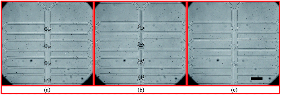
Therefore, the third version of the design was proposed after many tests and optimization to overcome the above drawbacks. The sketch of the design is shown in Fig. 1, which consists of two T-junction generators, a trapping chamber, a waste channel and a channel for removing dust inside the chip. The design is symmetric with respect to the centreline passing through the center of the continuous phase channel and the trapping chamber. The T-junction generator, as shown in Fig. 1(B), has a channel width of 120 μm and height 60 μm (channel height is uniform in the whole chip unless stated otherwise). Robustness is particularly emphasized in the channel design. First, the performance of the two droplet generators must be decoupled which is achieved by designing a long channel after each of the T-junctions. If it is too short, a droplet entering or exiting it will lead to significant fluctuation in the channel resistance, which will affect the droplet generation in the other T-junction path. Preliminary experimental testing indicated that the channel between the T-junction and trapping well on each side should be long enough to contain at least 40–50 droplets to damp the fluctuation which is set to be 42 mm. This decoupling eliminates the need for synchronizing the two droplet generation processes as in the previously reported designs (shown in Fig. S1 and S2†) which is quite challenging from the practical point of view. Second, an intersection is added before the trapping wells shown in Fig. 1(C) with the left branch for disposing waste and the right for removing dust. At the beginning of droplet generation, droplets are not uniform due to unstable flow conditions. These undesired droplets are disposed through the left branch through which the waste in the trapping wells after each reaction, is also released into the waste reservoir. A pillar is added at the entrance of the left branch to prevent droplets from entering it during the trapping time. The right branch is designed to remove any dust inside the chip. Although pillars are added in the entrance to filter the fluids, small pieces of PDMS inside the chip may still block the channel. High pressure is applied to remove the dust through this channel, where the channel width is set to be larger than the other three channels so that the dust can be easily removed (the right channel width is set to 150 μm, the others are set to 120 μm). The downstream channel is set to guide droplets into the trapping wells. The trapping design shown in Fig. 1(D) consists of two trapping wells and two bypass channels. Each bypass channel has a length of 4000 μm, and width of 120 μm. The trapping wells as shown in Fig. 1(E), have a diameter of 170 μm, and the distance between the two centres is 160 μm, which is slightly smaller than the trapping well diameter. Therefore, the two circles intersect and form a gap between them. The gap width at the intersection is 57.4 μm. The gap between each pillar is set to be 25 μm. The channel width of each branch is set to be 120 μm except otherwise stated.
 | ||
| Fig. 1 Sketch of the third version of the design for trapping two streams of droplets. (A) Overview of the chip design. The design is symmetric and has two separate T-junction droplet generators with exactly the same channel dimensions. (B) T-junction droplet generator for reagent 1 with channel height 60 μm, channel width of 120 μm for oil and reagent 1. (C) An intersection: the left channel is used to dispose sample waste; the right remove dust inside the microfluidic chip, and the downstream trap droplets. (D) Trapping design for trapping droplets from two droplet streams. The channel of sample waste has the same dimensions as the trapping channel. An array of trapping wells can be integrated into the flow stream depending on requirements. (E) Dimensions of two trapping wells. Inlet channel width keeps the same as upstream channels, 120 μm; trapping well diameter, 170 μm; distance between two centres, 160 μm; gap width at the intersection of the two wells, 57.4 μm; and gap width between each pillar, 25 μm. Compared to the other two designs, the third version minimizes the influence of two droplet generators on each other, enabling production of more monodispersed droplets. | ||
When a droplet from one stream (e.g. a droplet from stream 1) reaches the trapping channel, it will enter the trapping well because the resistance of the bypass channel is set to be higher than that of the trapping well. After being trapped, the droplet will stay inside the trapping well due to the interfacial tension and dramatically increase the resistance of the trapping well. The droplets behind the trapped one will enter the bypass channel then. When a droplet from the other stream (stream 2) reaches the trapping channel, it will also enter the other trapping well and merge with the trapped droplet from stream 1. Meanwhile, the reaction starts. The merged droplets mix fast within several seconds due to the disturbance induced by the droplets coming or leaving the main channels connected with the trapping wells.
The suggested operation steps for a typical chemical or biological reaction are summarized as follows:
1. Remove all the dust inside the chip by pumping oil with high pressures (1 bar in our experimental setup) from all of the inlets and outlets except the dust outlet, which is then blocked after dust removal.
2. Fill the sample inlets with reagent 1 and reagent 2 respectively and apply the estimated pressures at all the inlets and Outlet 1 to generate droplets and pump them into the waste channel towards Outlet 2. In general, the system takes a bit time to stabilize and generate uniform droplets. Non-uniform droplets should be eliminated for quantitative analysis which is realized in this design by adding a sample waste channel. By applying a moderate pressure which may vary with designs at Outlet 1 during the initial period of droplet generation, the unstable droplets can be pumped into the sample waste channel. The pressure applied to Outlet 1 is then adjusted to a threshold that can prevent the droplet from going into the trapping channel but not significant back flow into the sample waste channel. The pressure values applied at Outlet 1 should be estimated based on eqn (16) and calibrated at the beginning by visualization to ensure all the droplets entering the waste channel. Once the applied pressure values are fixed, they can be saved for future use (this step only needs to be done once).
3. Once the generated droplets are uniform, the same amount of pressure as that applied to Outlet 1 is applied to Outlet 2 leaving Outlet 1 open to the air. The droplets start going to the trapping channel.
4. Use a microscope and a high speed camera to record the trapping and reaction process.
5. After the reaction is finished, apply a high pressure to Outlet 1 (1 bar) and no pressure in Outlet 2 to release the sample.
6. After releasing the sample in the trapping channel, repeat step 3–6 for a second reaction.
2.2 Design criteria
To develop an individual function such as droplet generation, or droplet trapping, the effects of all the influencing parameters such as channel dimensions, flow rate ratios and viscosity contrast on the function's performance should be tested. For the integration of multiple functions, however, the focus is shifted to testing of the global design ensuring that multiple functions work robustly in an integrated manner. This integration concern presents limitations to many operating parameters, such as the channel dimensions and network design. For example, to ensure two droplet generators work robustly, their operation should be decoupled which is ensured by designing a long channel hosting a sufficiently large number of droplets (>50) for each generator which will diminish the fluctuations in the hydrodynamic resistance induced by a droplet entering or existing the generator region. Varying channel height and width adds more complexity to the design and operation which is avoided. Similar strategies are applied for the choices of the channel dimensions as detailed later, which leaves the set of applied pressures as the only external control of the system performance.To successfully trap droplets in the trapping wells, two conditions must be satisfied: (i) when a droplet reaches the entrance of the trapping wells, it must enter the trapping well; and (ii) after a droplet gets trapped, the droplet cannot be pushed through any gap connected with the trapping well (there are three gaps shown in Fig. 1(E)). To consider these criteria in the design, one-dimensional (1D) circuit analysis model is used to assist the design. Fig. 2(A) illustrates the design of the trapping well region and the definition of the associated parameters and Fig. 2(B) shows the 1D circuit analysis model. Before the discussion of the design criteria, please note that the two trapping wells and their associated channel layouts are symmetric as shown in Fig. 1(A).
 | ||
| Fig. 2 (A) Definition of parameters of a trapping well unit. Pup and Pdown are the pressures at the up junction and down junction, respectively; Pj1 and Pj2 the pressures at the T-junctions of each stream, respectively; Ptrap1 and Ptrap2 the pressures at the front tip of the trapped droplets; Qmain_1 and Qmain_2 the flow rates in the main channels of each stream, respectively; Qbypass_1 and Qbypass_2 the flow rates in each bypass channel; Qtrap_1 and Qtrap_2 the flow rates in each trapping well; w the channel width; wi the width of the intersection gap between two trapping wells; wgap the width between each pillar; r the radius of the trapping well; L1 length of the trapping well; L2 length of gap between each pillar; Ljunction length of the junction that connects the two main channels of the two streams; and Lmain length of the main channel. (B) Equivalent fluidic circuit of a trapping well unit with fluidic resistors. | ||
 | (1) |
 | (2) |
Eqn (1) is accurate for any rectangular channel with h/w < 1, when Reynolds number is below ∼1000.40 Therefore, the pressure drop through bypass channel I without droplets can be calculated as:
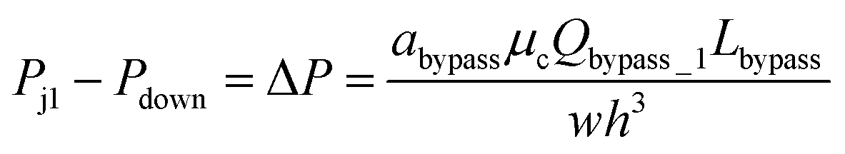 | (3) |
Each trapping well has an entrance on the left which connects to a short horizontal channel (referring to the main channel, Lmain, shown in Fig. 2(A)) through which a droplet can enter the well. It also has two gaps on the right connect to the right branch of the bypass channel. This two-gap design was found to be more robust than the one-gap design, which was reported previously by Tan et al.,41 because it can hold the trapped droplet while allowing more fluid going through the trap. The trapping well is circular in top view and rectangular in cross-section. We approximate the circular shape with the square that circumscribes it. This approximation only inputs negligible error (∼2%) in calculating the total hydrodynamic resistance of the trapping well region which consists of the channel between the T-junction and the entrance of the trapping well, the trapping well, and the gaps because the resistance of the trapping well is very small compared to the gaps, Rtrap ≪ Rgap. Due to the large resistance of the gaps, we can also estimate the pressure at the T-junction is equal to that of the entrance of the trapping well such that Pj1 ≈ Ptrap1, and Pj2 ≈ Ptrap2. Because the gap width is smaller than its height, we need to substitute the gap width as h, and gap height as w into eqn (1) to calculate Rgap. Therefore, the pressure drop through the trapping well can be also estimated as:
 | (4) |
Please note that eqn (4) considers trap II is filled with one droplet which results in a higher resistance for the trap region and lower flow rate towards trap I. Here, trap II is considered as blocked. Therefore, this is a more conservative design which means if this predicted design works for trapping droplets, the design would work even better for the scenario when trap II is not filled with a droplet. Combine eqn (3) and (4) we can obtain:
 | (5) |
Define non-dimensional forms:
 ,
,  ,
,  ,
,  ,
,  , and flow rate ratio
Then, eqn (5) can be rewritten into a non-dimensional form:
 | (6) |
In this design, the radius of the trapping well is set to be r = 0.7w (r = 85 μm) in order to allow the droplet to occupy most of the trapping well.  is set to be
  (L1 = 279 μm) so that the following droplets do not contact with the trapped droplet (avoid droplet merging).
  is set to be
  (L2 = 71 μm), and
  is set to be
  (wgap = 25 μm) due to fabrication limitation (if the pillars after the trapping well are too small, they could be peeled off from the silicon wafer). The actual channel dimensions are smaller than the designed since silicone oil swells PDMS channels. The actual channel dimensions (listed in Table 1) are measured after silicone oil sufficiently swells PDMS channels.
| Parameters | w (μm) | h (μm) | r (μm) | wi (μm) | wgap (μm) | L1 (μm) | L2 (μm) | Lbypass (μm) | Ljunction (μm) | Lmain (μm) |
|---|---|---|---|---|---|---|---|---|---|---|
| Nominal dimensions | 120 | 60 | 85 | 57.4 | 25 | 279 | 71 | 4000 | 50 | 210 |
| Actual dimensions | 100 | 53 | 75 | 66 | 15 | 291 | 74 | 4000 | 45 | 227 |
By substituting the actual channel dimensions into eqn (2), we can obtain: abypass = 17.93, atrap = 17.93, agap = 14.59. Substituting all the parameters into eqn (6), we can get:
 | (7) |
The final expression of the flow rate ratio, φ, is proportional to the bypass channel length,  . In order to trap a droplet in the trapping well, we must satisfy the criterion,
  . Therefore, the first condition must satisfy
  .
.
 | (8) |
Second, to prevent the trapped droplet from going through the gap between the pillars, the pressure drop through the trapping well and the pillars (ΔPd = Ptrap1 − Pdown ≈ Pj1 − Pdown) should be less than (or equal to) the Laplace pressure across the trapped droplet (ΔPLap2), which can be expressed as:
 | (9) |
Since  , eqn (9) can be simplified as,
 | (10) |
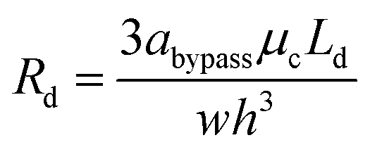
After a droplet gets trapped inside the trapping well, the following droplets will enter the bypass channel, which increases the hydrodynamic resistance of the bypass channel which can be estimated as:
 | (11) |
 | (12) |
 | (13) |
Droplet resistance is difficult to be accurately predicted without having some empirical data to work with, although several studies have experimentally studied the influence of the viscosity ratio, droplet speed, surface tension, droplet size and channel geometry on droplet resistance.42–44 Glawdel et al.45 proposed a suitable rule of thumb to estimate the droplet resistance, that is, each droplet will increase the resistance of the segment of channel it occupies by 2–5 times. Hence, we estimate Rd (we used 3 times) as:
 | (14) |
By substituting eqn (13) and (14) into eqn (10), we can obtain,
 | (15) |
After a droplet gets trapped, Qtrap_1 ≪ Qbypass_1, a small amount of fluid can still go through the trapping well due to the thin film between the droplet and channel wall (Qtrap_1 ≠ 0). Therefore, we have Qmain_1 = Qbypass_1 + Qtrap_1 > Qbypass_1. In order to ensure that the droplet remains in the trapping well, we set:
 | (16) |
If we satisfy eqn (16), eqn (15) is also satisfied because Qmain_1 > Qbypass_1. Qmain_1 can be expressed as:
| Qmain_1 = Ucwh | (17) |
 | (18) |
 is the capillary number of the continuous phase. One can see that the fluid properties such as the continuous phase viscosity and the interfacial tension for the pair of fluids also influence the design performance. The non-dimensional form of the second condition can be expressed as:
 | (19) |
 (Lbypass = 4000 μm, the ideal result calculated based on eqn (6) is Lbypass = 2800 μm) in order to make sure the droplet can directly enter the trapping well. By estimating the droplet length
  and the spacing
  , we can calculate the capillary number range that can allow droplets to remain inside the trapping wells, Ca ≤ 0.0033, when
  , and Ca ≤ 0.0037 when
  by using eqn (19).
• The length of each main channel between the two trapping well units should be much less than the droplet spacing to minimize the unbalance of the main channel resistances between two flow streams.
• There exists a minimum bypass channel length that ensures the droplet to be trapped.
• Reducing the bypass channel length can expand the range of capillary number, but the bypass channel length should be larger than the minimum required value.
• Increasing the channel height or reducing the gap width can also expand the range of capillary number, but the ratio  should be limited, it is hard to fabricate the gap when
  .
.
• Increasing the droplet spacing can also expand a larger capillary number range.
3 Experiments
3.1 Materials and chip fabrication
For all the experiments, two types of silicone oil (DC200, Sigma Aldrich) with a viscosity of 5 cSt and 10 cSt, respectively, were used as the continuous phase to consider the viscosity effect. Ultrapure water was used as reagent I, and Methylene Blue with a concentration of 1 mg mL−1 (diluted in ultrapure water) was used as reagent II to create a phase contrast in order to demonstrate the merging and mixing processes. No surfactant was added to any of the fluids.Microfluidic chips were fabricated using polydimethylsiloxane (PDMS) by standard soft-lithography techniques. A master was first fabricated by coating SU8-2025 (MICRO CHEM) on a silicon wafer. After being baked on a hot plate with 95 °C, the silicon wafer was then covered by a mask with the channel design, exposed under UV light with a controlled dose and baked on a hot plate again at 95 °C. Finally, the master was washed in SU-8 developer and ready to use. PDMS was mixed with a base/curing agent ratio of 10/1, and put into a vacuum oven to remove bubbles created during mixing. After that, PDMS was poured onto the master and put on the 95 °C hot plate for baking at least 2 hours. Then, the PDMS mold was bonded to a glass slide coated with a thin layer of PDMS using oxygen plasma. The surface of PDMS is naturally hydrophobic, but it will turn to hydrophilic after plasma bonding. Therefore, the bonded chip was put on a 190 °C hot plate for baking at least 24 hours to turn back to hydrophobic for this study which uses oil as the continuous phase. Finally, the chip was ready for experiments after cooling down.
3.2 Experimental setup
The fluids were pumped by a high precision microfluidic pressure control system (MSFC 8C, Fluigent). Droplet generation, trapping, mixing and releasing were visualized using an inverted epifluorescence microscope (Eclipse Ti, Nikon) with 4× and 20× objectives and a high speed camera (Phantom v210, Vision Research). Different input pressures were applied to span the range of capillary number and flow rates. Instead of using multiple flow sensors to monitor the flow rate for each streams, we measured the average velocity of droplets when they reached the entrance of the trapping wells, based on which the average velocity of silicone oil was estimated by dividing droplet velocity with a slip factor. The slip factor is defined as, α = ud/uc, where ud and uc are the velocity of the dispersed and continuous phase, respectively.Vanapalli et al.44 found the slip factor α = 1.28 for all droplets that tested under the following conditions: droplet length varies from 1.5–7.2w (w is the channel width), two viscosity ratios 0.03 and 0.88 (the dispersed phase to the continuous phase) and capillary number from 0.001–0.01 without surfactant. All of our flow conditions fall into these ranges. Therefore, we used α = 1.28 to estimate the velocity of the continuous phase in our experimental results. ud can be directly measured from the captured videos.
3.3 Experimental results
 | ||
| Fig. 3 Two streams of droplets captured from the high-speed camera with an 4× objective under the conditions: Poil1 = 500 mbar, Poil2 = 500 mbar, Pwater = 440 mbar, Pdye = 440 mbar, Poutlet1 = 230 mbar, Poutlet2 = 0 mbar. Silicone oil with a viscosity of 5 cSt (5 cSt silicone oil density 0.913 g mL−1) was used as the continuous phase. (a) Water droplets with droplet length about 2w and spacing 28w, and (b) Methylene Blue dye droplets with droplet length 2w and spacing 19w where w is the channel width. The scale bar is 500 μm. | ||
 | ||
| Fig. 4 Droplet pairing and trapping process captured from high-speed camera using an 4× objective under the conditions: Poil1 = 500 mbar, Poil2 = 500 mbar, Pwater = 440 mbar, Pdye = 440 mbar, Poutlet1 = 0 mbar, and Poutlet2 = 230 mbar. Silicone oil with a viscosity of 5 cSt was used as the continuous phase. Droplets containing Methylene Blue dye are on the left side branch, and water droplets are on the right side branch. (a) Droplets are approaching the first trapping well. The Methylene Blue droplets have an average velocity of ud_dye = 13.9 mm s−1, and the water droplets ud_water = 15.8 mm s−1. The capillary number of the continuous phase are estimated as Cac_dye = 0.00118 and Cac_water = 0.00134, respectively; (b) the first pair of trapped droplets; (c) the second pair of trapped droplets; (d) the third pair of trapped droplets; (e) the forth pair of trapped droplets and (f) four pairs of droplets are fully mixed after 4.15 s. The scale bar is 500 μm. | ||
 | (20) |
 | ||
| Fig. 5 Droplet merging and mixing process in one of the four trapping wells captured from high-speed camera using an 20× objective under the conditions: Poil1 = 500 mbar, Poil2 = 500 mbar, Pwater = 440 mbar, Pdye = 440 mbar, Poutlet1 = 0 mbar, and Poutlet2 = 230 mbar. Silicone oil with a viscosity of 5 cSt was used as the continuous phase. The darker droplet is Methylene Blue, and the brighter droplet is pure water. (a) The two droplets start merging and (b)–(h) droplets mixing process after merging. Line grayscale values (range 0–255, 0 – black and 255 – white) are plotted in each figure cross the centre of the trapping well, which shows that the reagents are fully mixed after 4 s. The scale bar is 100 μm. | ||
When a water droplet enters one of the main channels (Fig. 5(b) and (e)), it increases the main channel resistance of the water droplet stream, which results in more silicone oil flowing into the other stream with dye droplets following the condition of Qtrap2 > Qtrap1. As the result, the pressure at the two traps are not equal (i.e. Ptrap2 > Ptrap1), which pushes the merged droplet towards the water droplet side (i.e. rdye > rwater), as shown in Fig. 5(b) and (e). Similarly, when a dye droplet enters one of the main channels, the trapped and merged droplet will be slightly pushed towards the dye side (i.e. rdye < rwater) as shown in Fig. 5(c) and (f). Because of the designed length of the main channel which can only contain no more than one droplet, the merged droplet constantly receives the disturbance enhancing the mixing within it while the pressure fluctuation is not large enough to push the merged droplets out of the trapping well. When both main channels contain one droplet (see Fig. 5(d)) or no droplet (see Fig. 5(g)), the resistances of the two streams are balanced, and the two trapped droplets have the same shape (i.e. rdye ≈ rwater).
After both of the droplets get trapped and merged, the Laplace pressure drop between the two droplets (see Fig. 5(b)) can be calculated using eqn (21):
 | (21) |
In order to quantify the degree of mixing as a function of time, we measured the mixing index of the captured cross-section images, which is defined by Imix = 1 − Is, where Is is the discrete intensity of segregation defined by Danckwerts:48
 | (22) |
Because a droplet is 3D curved, the boundary of the trapped droplets is darker than the inside area, which could affect our measurement. Therefore, we excluded the boundary when we measured the grayscale value of each pixel inside the trapped droplets as shown in Fig. 6(a). A Matlab code was written to identify the contour of the trapped droplet in each frame and measure the grayscale value of each pixel inside the red line. We measured the mixing index Imix along with time under three different incoming droplet velocities (see Fig. 6(b)). Experimental results indicate that the mixing index is a power function of time. When Imix reaches 0.98, the two reagents are considered to be well mixed. From Fig. 6(b), we can see that the reagents were well mixed at around t = 3 s, when both cases with Ud = 17.3 mm s−1 and Ud = 19.8 mm s−1, respectively. The reagents were well mixed at around t = 6 s, when Ud = 12.9 mm s−1. Therefore, increasing the droplet velocity (or capillary number) can improve the mixing process, because it increases the fluctuation frequency of the droplet shape.
 | ||
| Fig. 6 (a) Grayscale value measurement area, where the boundary was excluded. The scale bar is 100 μm. (b) Mixing index vs. time under different droplet average velocities. | ||
 | ||
| Fig. 7 Droplet releasing process captured from the high-speed camera using an 4× objective under the conditions: Poil1 = 500 mbar, Poil2 = 500 mbar, Pwater = 0 mbar, Pdye = 0 mbar, Poutlet1 = 1000 mbar and Poutlet2 = 0 mbar. Silicone oil with a viscosity of 5 cSt was used as the continuous phase. (a) Droplets trapped inside the trapping wells before releasing, (b) the trapped droplets that were about to be washed out of the trapping wells, and (c) the trapping wells after rinsed by silicone oil. The scale bar is 500 μm. | ||
:3 to 3:1, which creates 5 different reagent concentrations.
 | ||
| Fig. 8 Sketch of the trapping well design for trapping multiple droplets with a concentration gradient of reagents. The number of trapped droplets ratio in a trapping well varies from 1:3 to 3:1, which creates 5 different reagent concentrations. | ||
The experimental trapping process is shown in Fig. 9(a–h) while Fig. 9(i) shows mixing occurring inside the trapped droplets. The figure shows four trapping wells, and the merged droplet has a final Methylene Blue dye concentration of 33.3% (the third well from the top), 50.0% (the first well from the top), 66.7% (the second well from the top) and 75.0% (the fourth well from the top) of the original concentration. The determination of the concentration can be found in the ESI.† Fig. 9(j) shows the droplets are being released from the trapping wells.
 | ||
| Fig. 9 Droplet trapping and releasing process for generating a concentration gradient captured from the high-speed camera using an 4× objective under the setting conditions: Poil1 = 480 mbar, Poil2 = 480 mbar, Pwater = 440 mbar, Pdye = 450 mbar, Poutlet1 = 0 mbar and Poutlet2 = 170 mbar. (a)–(h) are for the droplet trapping process and (i) and (j) shows the droplet mixing and releasing. The demonstration of each function of this design can be found in Movie 1 (M1) in the ESI.† The scale bar is 500 μm. | ||
4 An application for drug discovery
Tau-peptide aggregation is a phenomenon related to neurodegenerative disorders such as Alzheimer's disease (AD).51Assays for screening drug compounds for AD treatment often involve the test of the concentration of tau-aggregation inhibitors such as hexapeptide Ac-VQIVYK-NH2 (AcPHF6), which is a model peptide to investigate tau-aggregation.52,53 A fluorescent indicator named Thioflavin-T (ThT) is used to quantify the aggregation process.54 Traditional efforts rely on 96-well plates55 which has proven successful, however, are associated with some drawbacks such as large reagent consumption (∼200 μL per well) and long reaction time (∼2 h).55 Droplet microfluidics in contrast is capable of address these drawbacks because of the small volume of each drop (pL to nL) and shortened reaction time (∼several minutes) enabled by enhanced mixing within droplets. The proposed design offers additional benefits for performing such an assay including accurate control of reaction time enabled by on-demand trapping, easy of repeating experiments enabled by on-demand releasing.
The anti-tau aggregation inhibitor and fluorescent dye chosen for this study were orange G and ThT, which are the same as the reported assay.55,56 Four different sets of experiments were performed including positive control (the buffer solution with AcPHF6 and ThT), negative control (the buffer solution with ThT only) and two concentrations of Orange G (the same solution as that for the positive control with added Orange G of 16.5 μM and 33 μM, respectively). The detailed concentrations of each compound in the merged droplet for each experiment is listed in Table 2. During the experiments, one stream of the dispersed phase contains freshly prepared aqueous AcPHF6 (Celtek Peptides) stock solution with a concentration of 0.12 mg mL−1 and the other contains the rest reagents. The PH value of PBS buffer stock solution was adjusted to 7.3 using HCl. A small amount of DMSO (Sigma Aldrich) was added to help dissolve orange G in solution. 10 cSt silicone oil was used as the continuous phase. Microfluidic pressure control system (MSFC 8C, Fluigent) was used to drive the flow. The sample reagents were loaded into 2 mL reservoirs (Fluiwell 4C, Fluigent), which were immersed into an ice-water bath to prevent peptide self-aggregation. The sample reagents were injected into the microfluidic device using black tubing with inner diameter of 100 μm (IDEX Health & Science) to save sample cost. The aggregation process was imaged using an inverted epifluorescence microscope (ECLIPSE Ti, Nikon) with a 10× objective and a high sensitivity CCD Camera (Retiga 2000R, QImaging). Fluorescence was monitored at a wavelength of 440 nm for excitation and 490 nm for emission using a fluorescence filter (CFP-HQ, Nikon). Each aggregation kinetics was monitored in two trapping wells simultaneously, and each experiment was duplicated. Therefore, each aggregation process was repeated four times. The exposure time was set to 100 ms and hardware gain 21.5 for all experiments. The mercury halide lamp (Intensilight C-HGFIE, Nikon) was shut down during idle time to reduce photo bleaching, which was automatically controlled by a software developed by Nikon.
| Experiment | AcPHF6 (mg mL−1) | ThT (μM) | Orange G (μM) | PBS buffer (mM) | DMSO (% (v/v)) |
|---|---|---|---|---|---|
| Positive control | 0.06 | 3.1 | — | 16.5 | <1% |
| 16.5 μM Orange G | 0.06 | 3.1 | 16.5 | 16.5 | <1% |
| 33 μM Orange G | 0.06 | 3.1 | 33 | 16.5 | <1% |
| Negative control | — | 3.1 | — | 16.5 | <1% |
Operation steps are the same as that described in Section 2.1. Before trapping droplets, droplet sizes from two streams are adjusted to be the same using the strategy explained earlier in order to obtain consistent results. Fig. 10 shows the fluorescent intensity change within the merged droplets over time. As expected, the positive control has the highest intensity and the inhibitor does suppress the aggregation reflected by the reduced fluorescent intensity compared to that of the positive control. In addition, the higher the inhibitor concentration, the less aggregation. The detailed tau-aggregation process over time can be found in Movie 2 (M2†).
 | ||
| Fig. 10 Fluorescent images of trapped droplets changing over time for four experiments using CFP Nikon fluorescence filter, 10× objective, 100 m exposure time and 21.5 hardware gain. | ||
Fig. 11 shows the effect of orange G on tau-hexapeptide aggregation. The intensity values were obtained by averaging the intensity of the entire merged droplet for a given time. As expected, in the absence of inhibitor, AcPHF6 aggregates rapidly as monitored by fluorescence intensity over 5 min and then decreases to a plateau because the aggregates started to dissociate and photo bleaching effects may also play a role. A significant decrease in fluorescence intensity was observed when orange G was added, indicating a decrease in AcPHF6 aggregation. In addition, AcPHF6 aggregation is also dependent on the inhibitor concentration. The trend of testing results agrees well with that using 96-well plate performed by Mohamed et al.55 The most notable difference compared with 96-well plate is that the reaction is much faster (5 min vs. 2 h) due to enhanced mixing. However, the plateau phase has very small deviation within ±5%. The detailed data from all experiments can be found in Fig. S5 in the ESI.†
 | ||
| Fig. 11 Effect of inhibitor Orange G on AcPHF6 aggregation measured by a software (NIS-Elements, Nikon). Each plot is averaged from four measurements with a deviation around ±5%. The intensity data are subtracted from the background intensity (before droplet merging) for each experiment. | ||
Since the reaction is rapid, this design provides a significant advantage over other designs in controlling the reaction start time by separating two reagents and merging them on demand. Most of the previously reported droplet microfluidic devices cannot precisely control the reaction start time because two reagents are in contact when forming a co-flowing stream before droplet generation.
5 Conclusion
In this work, a microfluidic chip design that integrates droplet generation, pairing, trapping, merging, mixing, and releasing was proposed. The criteria of this design for realizing these functions in a robust manner were analysed and verified by experiments. This design's robustness is largely contributed by the eliminate of the need for synchronization of droplet frequency, spacing or velocity and the decoupling between each function. The entire chip operation is relying on liquid flow control involving no electrodes, magnets or any other moving parts. This design allows the monitoring of the merging of droplets and thus the precise control of reaction time. Experiments confirmed that homogenous mixing could be achieved as fast as several seconds taking advantage of the disturbance to the merged droplet shape by the droplets entering and exiting the main channel. In addition, a modified trapping well design can trap multiple droplets, which can generate a reagent concentration gradient. Finally, this design was used to test a tau-hexapeptide aggregation inhibitor relative to AD disease, and significantly reduced the reaction time compared to traditional 96-well plate (5 min vs. 2 hours) and sample cost (nL vs. μL). This design can be also applied in many other chemical or biological reactions.Acknowledgements
The authors acknowledge the Natural Science and Engineering Research Council of Canada, Canada Research Chair program, Canada Foundation for Innovation, and University of Waterloo for research grants to C. L. Ren.Notes and references
- A. J. DeMello, Nature, 2006, 442, 394–402 CrossRef CAS PubMed
.
- K. V. I. S. Karan and R. Prakash, Sensors, 2014, 14, 23283–23306 CrossRef PubMed
- A. M. Nightingale, T. W. Phillips, J. H. Bannock and J. C. de Mello, Nat. Commun., 2014, 5, 3777 CrossRef CAS PubMed
- G. T. Vladisavljević, N. Khalid, M. a. Neves, T. Kuroiwa, M. Nakajima, K. Uemura, S. Ichikawa and I. Kobayashi, Adv. Drug Delivery Rev., 2013, 65, 1626–1663 CrossRef PubMed
- O. J. Dressler, R. M. Maceiczyk, S. I. Chang and A. J. deMello, J. Biomol. Screening, 2014, 19, 483–496 CrossRef PubMed
- S. Y. Teh, R. Lin, L. H. Hung and A. P. Lee, Lab Chip, 2008, 8, 198–220 RSC
- R. Seemann, M. Brinkmann, T. Pfohl and S. Herminghaus, Rep. Prog. Phys., 2012, 75, 016601 CrossRef PubMed
- T. Thorsen, R. W. Roberts, F. H. Arnold and S. R. Quake, Phys. Rev. Lett., 2001, 86, 4163–4166 CrossRef CAS PubMed
- S. L. Anna, N. Bontoux and H. A. Stone, Appl. Phys. Lett., 2003, 82, 364 CrossRef CAS
- Z. Li, A. M. Leshansky, L. M. Pismen and P. Tabeling, Lab Chip, 2015, 15, 1023–1031 RSC
- Y. Ding, X. C. I. Solvas and A. deMello, Analyst, 2015, 140, 414–421 RSC
- V. Chokkalingam, S. Herminghaus and R. Seemann, Appl. Phys. Lett., 2008, 93, 254101 CrossRef
- B. Ahn, K. Lee, H. Lee, R. Panchapakesan and K. W. Oh, Lab Chip, 2011, 11, 3956–3962 RSC
- T. Glawdel, C. Elbuken and C. Ren, Lab Chip, 2011, 11, 3774–3784 RSC
- L. Frenz, J. Blouwolff, A. D. Griffiths and J. C. Baret, Langmuir, 2008, 24, 12073–12076 CrossRef CAS PubMed
- P. M. Korczyk, L. Derzsi, S. Jakieła and P. Garstecki, Lab Chip, 2013, 13, 4096–4102 RSC
- Y. Bai, X. He, D. Liu, S. N. Patil, D. Bratton, A. Huebner, F. Hollfelder, C. Abell and W. T. S. Huck, Lab Chip, 2010, 10, 1281–1285 RSC
- A. Huebner, D. Bratton, G. Whyte, M. Yang, A. J. Demello, C. Abell and F. Hollfelder, Lab Chip, 2009, 9, 692–698 RSC
- W. Shi, J. Qin, N. Ye and B. Lin, Lab Chip, 2008, 8, 1432–1435 RSC
- L. Mazutis and A. D. Griffiths, Lab Chip, 2012, 12, 1800–1806 RSC
- I. Akartuna, D. M. Aubrecht, T. E. Kodger and D. A. Weitz, Lab Chip, 2015, 15, 1140–1144 RSC
- M. Sesen, T. Alan and A. Neild, Lab Chip, 2014, 14, 3325–3333 RSC
- X. Niu, S. Gulati, J. B. Edel and A. J. deMello, Lab Chip, 2008, 8, 1837–1841 RSC
- A. Liau, R. Karnik, A. Majumdar and J. H. D. Cate, Anal. Chem., 2005, 77, 7618–7625 CrossRef CAS PubMed
- A. Sciambi and A. R. Abate, Lab Chip, 2015, 15, 47–51 RSC
- A. C. Hatch, A. Patel, N. R. Beer and A. P. Lee, Lab Chip, 2013, 13, 1308–1315 RSC
- K. Ahn, C. Kerbage, T. P. Hunt, R. M. Westervelt, D. R. Link and D. a. Weitz, Appl. Phys. Lett., 2006, 88, 024104 CrossRef
- B. Zheng, J. D. Tice, L. S. Roach and R. F. Ismagilov, Angew. Chem., Int. Ed. Engl., 2004, 43, 2508–2511 CrossRef CAS PubMed
- C. G. Yang, Y. F. Wu, Z. R. Xu and J. H. Wang, Lab Chip, 2011, 11, 3305–3312 RSC
- I. Shestopalov, J. D. Tice and R. F. Ismagilov, Lab Chip, 2004, 4, 316–321 RSC
- R. F. Shepherd, J. C. Conrad, S. K. Rhodes, D. R. Link, M. Marquez, D. A. Weitz, J. A. Lewis, P. Program, V. Di and C. Road, Langmuir, 2006, 18, 8618–8622 CrossRef PubMed
- A. R. Abate, T. Hung, P. Mary, J. J. Agresti and D. A. Weitz, Proc. Natl. Acad. Sci. U. S. A., 2010, 107, 19163–19166 CrossRef CAS PubMed
- Y. Wang, E. Tumarkin, D. Velasco, M. Abolhasani, W. Lau and E. Kumacheva, Lab Chip, 2013, 13, 2547–2553 RSC
- F. Scheiff, M. Mendorf, D. Agar, N. Reis and M. Mackley, Lab Chip, 2011, 11, 1022–1029 RSC
- C. Soto, Nat. Rev. Neurosci., 2003, 4, 49–60 CrossRef CAS PubMed
- X. Niu, F. Gielen, J. B. Edel and A. J. Demello, Nat. Chem., 2011, 3, 437–442 CrossRef CAS PubMed
- T. Glawdel, C. Elbuken, L. E. J. Lee and C. L. Ren, Lab Chip, 2009, 9, 3243–3250 RSC
- O. J. Miller, A. El Harrak, T. Mangeat, J. C. Baret, L. Frenz, B. El Debs, E. Mayot, M. L. Samuels, E. K. Rooney, P. Dieu, M. Galvan, D. R. Link and A. D. Griffiths, Proc. Natl. Acad. Sci. U. S. A., 2012, 109, 378–383 CrossRef CAS PubMed
- L. H. Hung, K. M. Choi, W. Y. Tseng, Y. C. Tan, K. J. Shea and A. P. Lee, Lab Chip, 2006, 6, 174–178 RSC
- C. J. Morris and F. K. Forster, Exp. Fluids, 2004, 36, 928–937 CrossRef
- W. H. Tan and S. Takeuchi, Proc. Natl. Acad. Sci. U. S. A., 2007, 104, 1146–1151 CrossRef CAS PubMed
- V. Labrot, M. Schindler, P. Guillot, A. Colin and M. Joanicot, Biomicrofluidics, 2009, 3, 12804 CrossRef PubMed
- S. S. Bithi and S. A. Vanapalli, Biomicrofluidics, 2010, 4, 44110 Search PubMed
- S. A. Vanapalli, A. G. Banpurkar, D. van den Ende, M. H. G. Duits and F. Mugele, Lab Chip, 2009, 9, 982–990 RSC
- T. Glawdel and C. L. Ren, Microfluid. Nanofluid., 2012, 13, 469–480 CrossRef CAS
- A. D. Stroock, S. K. W. Dertinger, A. Ajdari, I. Mezic, H. A. Stone and G. M. Whitesides, Science, 2002, 295, 647–651 CrossRef CAS PubMed
- C. De Loubens, R. G. Lentle, C. Hulls, P. W. M. Janssen, R. J. Love and J. P. Chambers, PLoS One, 2014, 9, 95000 Search PubMed
- P. V. Danckwerts, Appl. Sci. Res., Sect. A, 1952, 3, 279–296 Search PubMed
- O. J. Miller, A. El, T. Mangeat, J. Baret, L. Frenz, B. El, E. Mayot, M. L. Samuels, E. K. Rooney, P. Dieu, M. Galvan, D. R. Link and A. D. Griffiths, Proc. Natl. Acad. Sci. U. S. A., 2012, 109, 378–383 CrossRef CAS PubMed
- C. G. Yang, Z. R. Xu, A. P. Lee and J. H. Wang, Lab Chip, 2013, 13, 2815–2820 RSC
- E. F. Cohen and J. W. Kelly, Nature, 2003, 426, 905–909 CrossRef PubMed
- M. R. Sawaya, S. Sambashivan, R. Nelson, M. I. Invanova, S. A. Sievers, M. I. Apostol, M. J. Thompson, M. Balbirnie, J. W. Wiltzius, H. T. McFarlane, A. O. Madsen, C. Riekel and D. Eisenberg, Nature, 2007, 447, 453–457 CrossRef CAS PubMed
- S. A. Sievers, J. Karanicolas, H. W. Chang, L. Jiang, O. Zirafi, J. T. Stevens, J. Munch, D. Baker and D. Eisenberg, Nature, 2011, 475, 96–100 CrossRef CAS PubMed
- S. Hudson, H. Ecroyd, T. Kee and J. Carver, FEBS J., 2009, 276, 5960–5972 CrossRef CAS PubMed
- T. Mohamed, T. Hoang, M. Jelokhani-Niaraki and P. Rao, ACS Chem. Neurosci., 2013, 4, 1559–1570 CrossRef CAS PubMed
- M. Courtney, X. Chen, S. Chan, T. Mohamed, P. Rao and C. L. Ren, Anal. Chem., 2017, 89, 910–915 CrossRef CAS PubMed
Footnote |
| † Electronic supplementary information (ESI) available. See DOI: 10.1039/c7ra02336g |
| This journal is © The Royal Society of Chemistry 2017 |