
 Open Access Article
 This Open Access Article is licensed under a
 Creative Commons Attribution 3.0 Unported Licence
Response surface methodology as a powerful tool to optimize the synthesis of polymer-based graphene oxide nanocomposites for simultaneous removal of cationic and anionic heavy metal contaminants†
Jem Valerie D. Perezab,
Enrico T. Nadresa,
Hang Ngoc Nguyena,
Maria Lourdes P. Dalidab and
Debora F. Rodrigues *a
*a
aDepartment of Civil and Environmental Engineering, University of Houston, Houston, Texas 77204-5003, USA. E-mail: dfrigirodrigues@uh.edu
bDepartment of Chemical Engineering, University of the Philippines, 1101 Diliman, Quezon City, Philippines
First published on 28th March 2017
Abstract
Nanocomposites containing graphene oxide (GO), polyethyleneimine (PEI), and chitosan (CS) were synthesized for chromium(VI) and copper(II) removal from water. Response surface methodology (RSM) was used for the optimization of the synthesis of the CS–PEI–GO beads to achieve simultaneous maximum Cr(VI) and Cu(II) removals. The RSM experimental design involved investigating different concentrations of PEI (1.0–2.0%), GO (500–1500 ppm), and glutaraldehyde (GLA) (0.5–2.5%), simultaneously. Batch adsorption experiments were performed to obtain responses in terms of percent removal for both Cr(VI) and Cu(II) ions. A second-order polynomial equation was used to model the relationship between the synthesis conditions and the adsorption responses. High R2 values of 0.9848 and 0.8327 for Cr(VI) and Cu(II) removal, respectively, were obtained from the regression analyses, suggesting good correlation between observed experimental values and predicted values by the model. The optimum bead composition contained 2.0% PEI, 1500 ppm GO, and 2.08% GLA, and allowed Cr(VI) and Cu(II) removals of up to 91.10% and 78.18%, respectively. Finally, characterization of the structure and surface properties of the optimized CS–PEI–GO beads was carried out using X-ray diffraction (XRD), porosity and BET surface area analysis, scanning electron microscopy (SEM), Fourier transform infrared spectroscopy (FTIR), and X-ray photoelectron spectroscopy (XPS), which showed favorable adsorbent characteristics as given by a mesoporous structure with high surface area (358 m2 g−1) and plenty of surface functional groups. Overall, the synthesized CS–PEI–GO beads were proven to be effective in removing both cationic and anionic heavy metal pollutants.
1. Introduction
Wastewater is a necessary by-product of human activities. However, some industries, such as mining and electroplating, discharge effluents containing high levels of heavy metals, such as Cr(VI) and Cu(II), which are non-biodegradable and tend to accumulate in living organisms.1 These metals can pose serious threats to human health and the environment since they are toxic to living beings. Therefore, it is absolutely necessary to cleanse wastewater streams of heavy metals before disposal in the environment.Among the current treatment techniques used to separate heavy metals from wastewater, adsorption is preferred because of its advantages of low initial cost, flexibility, simplicity of design, ease of operation, and minimal sludge production.2 The main requirements for an efficient adsorbent are high capacity and fast adsorption. This can be achieved if the adsorbent has large surface area and plenty of adsorption sites.3 Unfortunately, most adsorbents rarely possess both properties at the same time. Hence, there is need for research of new adsorbents incorporating these key characteristics for a better adsorption of diverse heavy metals.3–5
Recent studies in nanotechnology highlight the strong adsorption abilities of graphene oxide (GO), making it an excellent adsorbent for heavy metals in itself or enhancers of other materials.6,7 GO possesses a large surface area and has numerous oxygen-containing functional groups protruding from the graphene backbone that make metal cations bind readily to it. However, GO is hydrophilic and very small, therefore it cannot be easily separated from water even by filtration or centrifugation, which limits its application in water treatment.8 In light of this, GO can be incorporated into polymer networks to maximize its properties and produce polymer nanocomposites with improved adsorption capabilities for a wide range of target pollutants.9,10
Chitosan, a known biosorbent, is a derivative of chitin, which is the second most abundant natural polymer after cellulose. Chitosan has been explored extensively for many applications because of its low cost, hydrophilicity, biodegradability, and antimicrobial properties.11 It has been proven to be an effective adsorbent for heavy metals because of the amino and hydroxyl functional groups present in its structure.12 Amine groups form complex reactions with cationic metal ions, while anionic ions are adsorbed by electrostatic attraction.13 Despite the favorable characteristics of chitosan, it has poor mechanical strength and is unstable, which hinder its practical applications.14 These drawbacks can be solved by physical and chemical modifications, such as gel formation into porous beads, reaction with cross-linking agents, and incorporation of nanomaterials. The bead formation provides better adsorption ability compared to its flakes/powder form due to decrease in crystallinity and expansion of the chitosan polymer network.15,16 Incorporation of nanomaterials, such as GO, has produced beads and chitosan gels with superior mechanical strength,17 and also with significantly improved adsorption capacities of the new polymer nanomaterials toward cationic heavy metals.9 Additionally, cross-linking agents, such as glutaraldehyde (GLA), formaldehyde, and epichlorohydrin (ECH), are used to chemically modify chitosan and make it insoluble and applicable in acidic conditions.18 However, most of these agents, even ECH, tend to react with the amine groups of chitosan. This reaction decreases the availability of adsorption sites.15 Thus, introduction of more functional groups have been achieved by blending chitosan with other polymers. These polymer composites have been shown to maintain or even improve the adsorption capacity of chitosan derivatives toward heavy metals.19–21
Polyethyleneimine (PEI), a polymer containing many primary and secondary amines,13 has been gaining attention as a polymer-based adsorbent for wastewater and heavy metal treatment.22–24 Because of the large number of amine groups in its structure, PEI has been shown to be a good chelating polymer for metal cations specifically Cu2+.25,26 Modification of CS beads with PEI significantly increased the amine groups present in the new material, giving it better adsorption capacity towards Cu2+ ions compared to unmodified beads.27 In addition, PEI can easily be protonated at low pH conditions, making it favorable for anionic metal ions, such as Cr(VI), via electrostatic attraction.13,28
In this study, polyethyleneimine (PEI) and GO were incorporated for the first time into the chitosan matrix to produce CS–PEI–GO porous nanocomposite beads. The unique properties of PEI and GO to bind to anionic and cationic contaminants, respectively, were optimized using Response Surface Methodology (RSM) to generate a multifunctional material. We hypothesize that the favorable properties of each individual components of the nanocomposite and the many and different functional groups in the final nanocomposite bead will produce a stable nanocomposite material with superior capacity to adsorb both anionic Cr(VI) and cationic Cu(II) ions. The optimum composition of the beads for maximum removal of both metals was determined with the response surface methodology (RSM). RSM experimental design was used in this study to evaluate the relationship between the different factors and responses with a smaller number of experimental runs, while also considering the interaction effects among the independent variables.29 RSM has been widely utilized for design of experiments and optimization processes by combining mathematical modeling and statistical techniques.30,31 Synthesis conditions of CS–PEI–GO nanocomposites in terms of concentrations of PEI, GO, and cross-linking agent GLA were investigated and optimized for maximum removal efficiency. The final optimized nanocomposite was also fully characterized.
2. Experimental section
2.1. Materials
The graphite (<45 μm) used for the synthesis of graphene oxide was purchased from Sigma-Aldrich. Low molecular weight chitosan (CS) was also purchased from Sigma-Aldrich. The sodium nitrate, potassium permanganate, potassium dichromate, copper(II) chloride, branched polyethyleneimine (50% wt% in H2O; MW ∼ 750![[thin space (1/6-em)]](https://www.rsc.org/images/entities/char_2009.gif) 000) and 25% glutaraldehyde solution (v/v) were also purchased from Sigma-Aldrich. Other chemicals such as sodium hydroxide, sulfuric acid, hydrochloric acid, and hydrogen peroxide solution were obtained from Fisher Scientific. All reagents used were of analytical grade, and all aqueous solutions were prepared using deionized (DI) water, unless indicated otherwise.
000) and 25% glutaraldehyde solution (v/v) were also purchased from Sigma-Aldrich. Other chemicals such as sodium hydroxide, sulfuric acid, hydrochloric acid, and hydrogen peroxide solution were obtained from Fisher Scientific. All reagents used were of analytical grade, and all aqueous solutions were prepared using deionized (DI) water, unless indicated otherwise.
2.2. Synthesis and characterization of GO
500 rpm for 5 min. The collected brown precipitate was then mixed with distilled water and centrifuged again under the same conditions. The washing process was repeated until the pH of the resulting supernatant became neutral. The precipitate was re-suspended in 2 L distilled water then sonicated for 8 h for exfoliation of graphite oxide. The sonicated solution was settled overnight, then decanted and freeze-dried to obtain pure GO powder.2.3. Synthesis of CS–PEI–GO beads using RSM
2.4. Experimental design and statistical analysis
The effects of the synthesis conditions on the heavy metal removal efficiencies of the beads were investigated by employing a three-factor and three-level Box-Behnken Design with two output responses. The concentrations of PEI (X1), GO (X2), and crosslinking agent GLA (X3) were used as the independent input variables/factors, and the percentage removal of Cr(VI) (Y1) and Cu(II) (Y2) were taken as the output responses. The range of concentrations/levels for the independent input factors were determined by performing preliminary investigations based on the successful synthesis of the beads. Coded and actual levels of each factor are presented in Table 1. Design Expert software (Stat-Ease Inc., Minneapolis, USA) was used to design the total number of experiments (15 runs with three center point replicates) and analyze the experimental data. All runs were randomized and performed in triplicate.| Independent Variables | Levels | ||
|---|---|---|---|
| −1 | 0 | +1 | |
| X1, PEI concentration (%) | 1.0 | 1.5 | 2.0 |
| X2, GO concentration (ppm) | 500 | 1000 | 1500 |
| X3, GLA concentration (%) | 0.5 | 1.5 | 2.5 |
The mathematical relationships of the independent variables with the obtained responses were established by fitting the experimental data to a second-order polynomial equation as given by eqn (1)
 | (1) |
Statistical analysis was done to evaluate the significance of each term in the model in terms of Analysis of Variance (ANOVA), with probability values established at P ≤ 0.05. The adequacy and predictability of the model was also tested using the lack-of-fit criterion, coefficient of determination R2, adequate precision, and residual diagnostics.
2.5. Optimization of the nanocomposite synthesis
To obtain the best composition of the CS–PEI–GO beads, Cr(VI) and Cu(II) responses were maximized by performing numerical optimization of the generated models based on a desirability function. Beads with the resulting optimum composition were synthesized and additional validation experiments were performed to verify the accuracy of the model prediction. All statistical analyses and optimization were done using the Design Expert software.2.6. Batch adsorption experiments for heavy metal removal
To determine the heavy metal removal efficiency of the synthesized CS–PEI–GO with different compositions and the optimized bead composition, batch adsorption experiments were performed at 25 °C in triplicate. Stock heavy metal solutions (1000 ppm) were prepared by dissolving appropriate amounts of K2Cr2O7 and CuCl2·2H2O in DI water. The pH was maintained at pH 5.5 to prevent metal precipitation. Working concentrations of 10 ppm Cr(VI) and Cu(II) solutions were obtained by serial dilutions of the stock solutions.The CS–PEI–GO beads (0.5 g) were added to heavy metal solutions (20 mL, 10 ppm) in 50 mL conical tubes. The solutions with the beads were mixed for 24 h at 130 rpm. The beads were then removed and the concentrations of the Cr(VI) and Cu(II) ions left in the solutions after the adsorption process were measured using a flame atomic adsorption spectrometer (AAnalyst 200, Perkin Elmer). The removal efficiency of the beads was calculated using eqn (2)
 | (2) |
2.7. Characterization of the optimized CS–PEI–GO beads
The synthesized CS–PEI–GO beads with the best composition were characterized in terms of surface properties. Prior to characterization, the beads were freeze-dried for 24 h. The beads were characterized by FTIR, XPS and XRD, using the same conditions described above.The morphology of the synthesized beads were determined with Scanning electron microscopy (SEM). Prior to analysis, the freeze-dried beads were coated with a thin layer of gold using a Desk V sputter (Denton Vacuum, NJ). This step was to ensure that the surface was conductive and to protect the samples from the high energy beam of the instrument. The Brunauer–Emmett–Teller (BET) surface area and porosity measurements were done using an ASAP 2020 V4.02 analyzer (Micromeritics, USA). Nitrogen gas adsorption–desorption isotherms were measured at 77 K. Relative pressures of 0.05 to 0.25 were selected for the linear range of the BET method. Prior to measurement, the freeze-dried beads were degassed at 120 °C for 300 min. Chemical and thermal stability tests were also performed. Solubility experiments were done by placing 0.5 g beads into 20 mL of different solutions (0.1 M and 1 M HCl and NaOH, and 5% (v/v) acetic acid). The solutions were mixed for 24 h at 130 rpm and observed. For Thermogravimetric Analysis (TGA), freeze-dried beads were ground into powder and pre-weighed into an Al2O3 pan. Analysis was done under N2 atmosphere from 25 to 550 °C at a heating rate of 10 °C min−1.
3. Results and discussion
3.1. Characterization of GO
To confirm the successful synthesis of GO, several characterization analyses were performed. X-ray diffraction patterns of GO and graphite are shown in Fig. 1. A sharp diffraction peak at 2θ = 26.84° is observed for graphite, which corresponds to a d-spacing of 0.332 nm. On the other hand, GO exhibits a relatively broader diffraction peak at a lower angle of 2θ = 11.25°, with a corresponding d-spacing of 0.786 nm. The observed GO peak is due to graphite oxidation and is consistent with the known characteristic peak of GO,35 indicating that GO was successfully synthesized. Also, the absence of peak is observed for GO at about 26°, suggesting full oxidation of the synthesized product.36 Furthermore, the observed increase in the d-spacing of GO compared to that of graphite can be attributed to the presence of oxygen-containing functional groups.35,37 Because of these functional groups, water easily intercalates the layers of oxidized graphite, which also contributes to the increased d-spacing of GO.37 | ||
| Fig. 1 XRD spectra of graphite and GO. | ||
Raman spectroscopy, Fourier transform infrared spectroscopy (FTIR), and X-ray photoelectron spectroscopy (XPS) were done to further confirm the successful synthesis of GO, and the spectra are presented in the (ESI) (Fig. S1 and S2†).
3.2. Experimental design and statistical analysis
The components used in the synthesis of CS–PEI–GO beads, i.e. the concentration of PEI, GO, and GLA, were optimized with BBD. The BBD was chosen to design the CS–PEI–GO composition since it requires synthesis of fewer number of beads with different compositions to adequately explain the behavior of a three-factor and three-level system.38,39 Midpoints of the edges of a cube and replicates of the center point represent the combinations of bead components in this design. The combinations of the nanocomposite components can also be viewed as three interlocking 22 factorial designs and center point replicates.40 The sequence of experiments with the actual and predicted responses obtained from the runs are summarized in ESI Table S1.† Actual responses, i.e. heavy metal removal, represent average values of the results from triplicate experiments. To each set of responses obtained with the different beads synthesized, the proposed quadratic model was fitted to develop a correlation between the synthesis conditions and the metal removal efficiencies. The resulting second-order equations for Cr(VI) and Cu(II) removal in terms of coded factors are expressed by eqn (3) and (4), respectively.| Y1(% Cr(VI) removal) = 79.34 + 0.82x1 + 1.24x2 + 4.78x3 + 1.22x1x2 + 0.23x1x3 − 0.047x2x3 + 3.59x12 + 2.47x22 − 0.95x32 | (3) |
| Y2(% Cu(II) removal) = 61.34 + 2.27x1 + 6.87x2 − 5.09x3 + 2.61x1x2 + 1.04x1x3 + 1.84x2x3 + 4.30x12 + 2.57x22 + 2.43x32 | (4) |
The values and the signs of the coefficients obtained from the model equations allow the assessment of how each bead component influence the responses.41 Positive values for the coefficients indicate positive influence to the response, while negative values correspond to antagonistic effects.42 From eqn (3), it can be seen that all three factors have a positive effect on Cr(VI) removal. On the other hand, GLA concentration inhibits the removal of Cu(II), as seen in eqn (4). Additionally, the values of the coefficients suggest that GLA concentration has the largest effect on Cr(VI) removal, while GO concentration affects Cu(II) removal the most.
The significance of each term in the model equations was evaluated using Analysis of Variance (ANOVA), and the results are shown in ESI Tables S2 and S3† with high F values and low probability values as the significance criteria.41,43 Most of the variation in the results is not due to noise and can be explained by the model when the F value is large, and the corresponding probability value checks whether it is statistically significant.40 Probability values less than 0.05 suggest that the terms in the model are significant, while values greater than 0.1 suggest non-significant terms. From ESI Table S2,† the regression model F-value of 37.94 with a probability value of 0.0004 suggest that the model for Cr(VI) removal is highly significant, and that there is only 0.04% chance that the model F-value is due to random error. Also, x1x3 and x2x3 with probability values of 0.6265 and 0.9215 respectively, are the only non-significant terms. Furthermore, with the largest F-value of 223.42 and the smallest probability value of <0.0001, ANOVA confirms that the GLA concentration has the most significant effect on Cr(VI) removal. Finally, lack-of-fit tests are possible because of the three replicates of the center point in the design to account for the pure error of the system.40 From ESI Table S2,† it can be seen that the lack-of-fit value is 0.3003, indicating non-significance with respect to pure error. The non-significant lack-of-fit is good because it implies that the model can be used as a response predictor.
On the other hand, ANOVA results for Cu(II) removal (ESI Table S3†) show that the probability value of the model is 0.0142, indicating that the model is significant and that there is only 1.42% chance that the F-value of 8.68 is caused by noise. Also from ESI Table S3,† ANOVA confirms that GO concentration has the most significant effect on Cu(II) removal, as suggested by the largest F-value of 38.16 with corresponding probability value of 0.0016. However, interaction coefficients x1x2, x1x3, and x2x3, and second-order model terms x22 and x32 are not significant, with probability values of 0.1573, 0.5369, 0.2954, 0.1768, and 0.1983 respectively. The model's lack-of-fit value indicates that there is 8.30% chance that the lack-of-fit F-value is due to noise.
To improve the predictability of the responses, model reduction was done by eliminating the insignificant terms determined by ANOVA from eqn (3) and (4).34 The reduced model equations in terms of coded factors are given by eqn (5) and (6)
| Y1(% Cr(VI) removal) = 79.34 + 0.82x1 + 1.24x2 + 4.78x3 + 1.22x1x2 + 3.59x12 + 2.47x22 − 0.95x32 | (5) |
| Y2(% Cu(II) removal) = 64.20 + 2.27x1 + 6.87x2 − 5.09x3 + 3.94x12 | (6) |
The removal efficiencies as predicted by eqn (5) and (6) are presented in the last two columns of ESI Table S1.† The results show good correlation between the actual values and the predicted responses, as also shown in Fig. 2. The low standard deviations of the models (0.78% and 3.71% for Cr(VI) and Cu(II) response, respectively) also confirm the goodness of fit.
 | ||
| Fig. 2 Predicted versus actual response plots for (a) Cr(VI) and (b) Cu(II) removal. Good agreement between actual experimental responses and predicted responses by the reduced models is observed for both metals. Colored legends show low (blue) to high (red) values of responses. | ||
The coefficient of determination R2 evaluates how well the model can predict the response,34 and it shows good agreement between experimental and predicted values when R2 is close to 1.43 In this study, high R2 values of 0.9848 and 0.8327 for Cr(VI) and Cu(II), respectively, were obtained. This suggests that the models can explain 98.48% and 83.27% of the total variations in the responses. Additionally, adjusted R2 values were also calculated to correct for the sample size used and the number of terms in the models.34,41
Still, relatively high values of 0.9695 and 0.7657 for Cr(VI) and Cu(II) models, respectively, were obtained after correction, indicating that the models generated for the system design have good predictability. Another criterion considered is the adequate precision value, defined as the signal-to-noise ratio of the model.30,34 This value shows a comparison between the predicted response and the pure error of the prediction, and a ratio higher than 4 is desired.34,41 Obtained values of 24.140 and 11.696 for Cr(VI) and Cu(II), respectively, further justify that the models are adequate for predicting responses.
Additional evaluation of the adequacy of the models was done using residual diagnostics. It is estimated that the difference between the actual and predicted responses are normally distributed, as ideally represented by the residuals following a straight line in the normal probability plot.30,41 The results presented in ESI Fig. S3(a) and (b)† show that the data points are approximately linear for both responses, indicating that the residuals follow a normal distribution and that no transformation is required. Furthermore, the residual data points appear to be distributed randomly showing no pattern with the responses, as shown in ESI Fig. S3.† Also, no outliers are observed, as the residuals are scattered within a narrow range, less than the set limit of ±3.0. The diagnostics indicate that the generated BBD models are suitable for Cr(VI) and Cu(II) removal optimization.
 | ||
| Fig. 3 Cr(VI) surface plots. (a) The effects of PEI and GO concentration on Cr(VI) removal show upward curvature confirming significant positive quadratic terms from ANOVA results; (b) the effects of PEI and GLA concentration as well as (c) the effects of GO and GLA concentration show higher removals of Cr(VI) when GLA concentration is increased. | ||
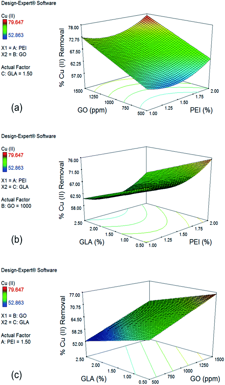 | ||
| Fig. 4 Cu(II) surface plots. (a) The effects of PEI and GO concentration on Cu(II) removal show upward curvature for PEI trend and also demonstrate large positive effect of GO; (b) the effects of PEI and GLA concentration show negative effect of GLA concentration; and (c) the effects of GO and GLA concentration show maximum increase in Cu(II) removal when GLA concentration is decreased and GO concentration is increased. | ||
Fig. 3b shows the effect of PEI and GLA concentration on % Cr(VI) removal with a constant GO concentration of 1000 ppm. Slight downward curvature of the GLA trend is in agreement with the negative quadratic term x32 of the reduced model. When GLA concentration is increased from 0.5 to 2.5% with 2.0% PEI, Cr(VI) removal is improved from 78.02% to 87.57%. Similar trend is observed for the effect of GO and GLA concentration on % Cr(VI) removal when PEI concentration is held constant at 1.5%, as shown in Fig. 3c. Cr(VI) removal increases from 77.32% to 86.87% when GLA concentration is increased from 0.5 to 2.5% at maximum GO concentration of 1500 ppm. Crosslinking with GLA yields imine bonds whose form is still cationic and could also participate in the electrostatic attraction of the Cr(VI) ions.46
In the case of Cu(II), the effect of PEI and GO concentration on % removal with a GLA concentration of 1.5% is shown in Fig. 4a. Upward curvature for the PEI concentration is explained by the significant quadratic term x12 of the reduced model. Increase in GO concentration from 500 to 1500 ppm significantly improves Cu(II) removal from 63.54% to 77.27%. This large effect is due to the coefficient of the term x2 in the reduced model having the largest positive value. Introduction of more GO and PEI resulted into more functional groups that are capable to adsorb Cu(II) ions. Although PEI addition makes the surface of the beads positive and therefore not favorable for Cu(II) adsorption because of electrostatic repulsion, analysis of the response plots still show increased removal for Cu(II) ions with further increase in PEI concentration due to addition of more amine groups which are primary sites for Cu(II) adsorption.
Fig. 4b shows the effect of PEI and GLA concentration on % Cu(II) removal with 1000 ppm GO. GLA concentration has a negative effect on % removal of Cu(II), as represented by the negative x3 term of the reduced model. Under constant PEI concentration of 2.0% and decreased concentrations of GLA from 2.5% to 0.5%, higher % removal of Cu(II) from 65.31% to 75.50% is achieved. This trend is opposite to that observed for Cr(VI) removal, and it could be explained by the difference in the mechanisms by which the two metal species are bound to the amino groups of PEI and chitosan. Cr(VI) ions are held by the adsorbent primarily via electrostatic attraction, while Cu(II) ions are held by complex formation with the primary amine groups on the surface of the beads.13 Crosslinking with GLA consumes some of the amine groups, resulting into the observed lower Cu(II) removal.
Finally, the effect of GO and GLA concentration on % removal of Cu(II) is shown in Fig. 4c with PEI concentration of 1.5%. The trend observed is linear since both the quadratic terms x22 and x32 were not significant from the ANOVA results. As mentioned earlier, maximum % removal of Cu(II) is achieved when GLA concentration is minimum and GO concentration is maximum. Increasing the GO concentration from 500 ppm to 1500 ppm and decreasing the GLA concentration from 2.5% to 0.5% resulted in a large increase of % Cu(II) removal from 52.24% to as high as 76.15%.
3.3. Optimization of the nanocomposite synthesis for the removal of heavy metals
The response surface analyses predicted optimum concentrations of PEI, GO, and GLA to result into maximum heavy metal removal efficiencies. Statistical analyses with RSM were done with Cr(VI) and Cu(II) separately, however, to produce a single type of adsorbent that could efficiently remove high amounts of both metal pollutants, numerical optimization was done using both Cr(VI) and Cu(II) responses. The numerical optimization was employed such that the concentrations of PEI, GO, and GLA were kept in range to ensure the successful synthesis of the beads, while both responses (Cr(VI) and Cu(II) removal) were maximized. A desirability function was used to perform the optimization, and the generated solution with the highest desirability value was chosen. The analysis determined that the optimum composition of the beads were 2.0% PEI and 1500 ppm GO, and the crosslinking GLA reagent should be at a concentration of 2.08%. The model predicted that this composition would result to 91.11% and 74.32% removal of Cr(VI) and Cu(II), respectively. Beads with this optimum composition were prepared using the same synthesis procedure, followed by adsorption experiments to verify the predictability of the model for each metal response. In addition, control beads (CS, CS–PEI, CS–GO) were also prepared using the corresponding optimum concentrations of each variable as determined by the optimization results. Validation results of the optimum conditions, as well as comparison with the control beads are shown in Fig. 5. Two-tailed t-test analysis (α = 0.05) was performed to determine if the values obtained are statistically different from each other. Calculated P values of 0.9929 and 0.2155 for Cr(VI) and Cu(II), respectively, confirm that there is no significant difference between experimental results from the optimized CS–PEI–GO beads and the predicted responses from the respective models. These results suggest that the model prediction is valid. Finally, it can be observed that both Cr(VI) and Cu(II) responses of the optimized CS–PEI–GO beads are higher than the responses of all the control beads, suggesting that the combination of all the starting materials (CS, PEI, and GO) in the beads indeed produces a more efficient adsorbent for both negatively-charged Cr(VI) and positively-charged Cu(II) pollutants.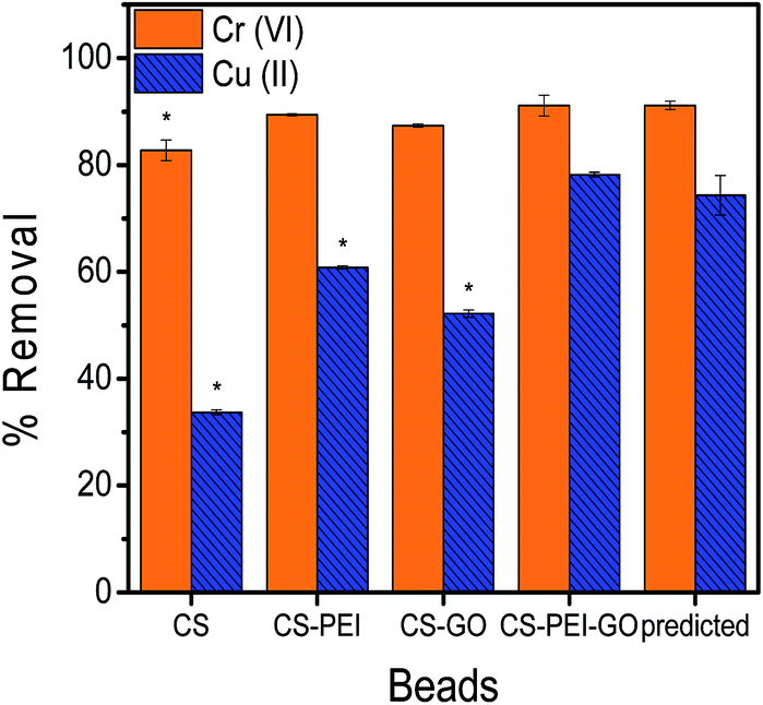 | ||
| Fig. 5 Validation of optimum conditions (*denotes statistically significant difference from CS–PEI–GO results). The results from validation experiments with optimized CS–PEI–GO beads are not statistically different from the responses as predicted by the respective models. Adsorption experiments were done with 10 ppm of 20 mL metal solutions at pH = 5.5 for 24 h contact time. | ||
3.4. Characterization of the optimized CS–PEI–GO beads
Fig. S4† shows a macro-image of the synthesized CS–PEI–GO beads with an average diameter of about 3 mm, confirming successful bead formation. In order to demonstrate successful synthesis and understand the physico-chemical properties of the new optimized CS–PEI–GO beads, FTIR and XPS were used to determine the functional groups in the new material and surface composition of the beads. The beads were further analyzed for chemical and thermal stability using solubility tests and TGA, as well as for crystallinity, porosity, and surface morphology using XRD, BET, and SEM analyses.The comparison of the FTIR spectra of pure/uncrosslinked CS, crosslinked CS, and CS–PEI–GO beads is presented in Fig. 6 to show changes with the functional groups present in the material. IR peaks of CS that are also present and unchanged in the other spectra appear at wavenumbers of 2877, 1375, and 1065 cm−1. These peaks can be attributed to the C–H stretch from CS backbone, C–H stretch from –NHCOCH3 group,47 and C–O–C stretch,48 respectively. Changes after crosslinking with GLA include a slight shift of the CS peak at 3361 cm−1 (assigned to –OH and –NH stretching vibrations) to 3369 cm−1. Also, CS peaks at 1651, 1594, and 1418 cm−1, which can be attributed to the carbonyl stretch of –NHCO– group (amide I),49 –NH bending of amine,48 and primary amine group,16 respectively, have disappeared in the spectra of the crosslinked CS. All these changes with –NH bands indicate the participation of amine groups in the crosslinking process. On the other hand, new peaks at 1653 and 1562 cm−1 are observed in the crosslinked CS spectrum. These two peaks can be attributed to imine (C![[double bond, length as m-dash]](https://www.rsc.org/images/entities/char_e001.gif) N) and ethylenic (CC) bonds, respectively, which confirm the successful crosslinking with GLA. Moreover, no unreacted aldehyde from GLA is observed, as given by the absence of a peak around 1720 cm−1, which suggests successful washes of the residual GLA from the beads.16,50 Changes upon addition of PEI and GO are observed by comparing the crosslinked CS and CS–PEI–GO spectra. The main functional groups commonly seen in GO are not visible because of the low GO content of the synthesized nanomaterial. The peak assigned to –OH and –NH stretch shifted to 3377 cm−1 and its intensity increased, suggesting the presence of more hydroxyl groups from GO and amine groups from PEI. The intensities of the peaks at 1654 and 1561 cm−1, which are assigned to the products of the crosslinking reaction with GLA, also increased due to more amine groups from PEI being converted to imine groups and paired with ethylenic double bonds from aldol condensation. Lastly, due to the incorporation of PEI in the nanomaterial, a shoulder peak at 1435 cm−1 assigned to primary amine groups is observed in the CS–PEI–GO spectrum, indicating the addition of more potential active sites for adsorption, hence achieving higher metal removals with PEI addition.
N) and ethylenic (CC) bonds, respectively, which confirm the successful crosslinking with GLA. Moreover, no unreacted aldehyde from GLA is observed, as given by the absence of a peak around 1720 cm−1, which suggests successful washes of the residual GLA from the beads.16,50 Changes upon addition of PEI and GO are observed by comparing the crosslinked CS and CS–PEI–GO spectra. The main functional groups commonly seen in GO are not visible because of the low GO content of the synthesized nanomaterial. The peak assigned to –OH and –NH stretch shifted to 3377 cm−1 and its intensity increased, suggesting the presence of more hydroxyl groups from GO and amine groups from PEI. The intensities of the peaks at 1654 and 1561 cm−1, which are assigned to the products of the crosslinking reaction with GLA, also increased due to more amine groups from PEI being converted to imine groups and paired with ethylenic double bonds from aldol condensation. Lastly, due to the incorporation of PEI in the nanomaterial, a shoulder peak at 1435 cm−1 assigned to primary amine groups is observed in the CS–PEI–GO spectrum, indicating the addition of more potential active sites for adsorption, hence achieving higher metal removals with PEI addition.
 | ||
| Fig. 6 FTIR spectra of pure/uncrosslinked CS, crosslinked CS, and CS–PEI–GO. | ||
Chemical and thermal stability tests were also performed to further confirm successful crosslinking and successful synthesis. Solubility tests with different solvents were performed and the results proved that the beads are insoluble in different acidic and basic solutions, as shown in ESI Table S4.† The good chemical stability of the beads can be attributed to the successful crosslinking reaction between GLA and the amine groups present in the beads. This stability over a wide pH range is favorable for the potential applicability of the beads to different types of wastewaters, as well as the possibility of regeneration of the beads using different desorption agents. TGA results presented in Fig. 7 show that all curves have an initial mass loss when heated to 100 °C due to evaporation of trapped water and moisture in the materials. Sharp weight loss of around 30% when GO was heated from 150 to 300 °C can be attributed to the pyrolysis of the oxygen-functional groups of GO.49 This decomposition for the synthesized beads happened gradually and was observed to start at a higher onset temperature (250 °C), an indication of the enhanced thermal stability of the CS–PEI–GO beads due to the strong interaction between the functional groups of GO and the polymers in the beads. Lower weight% observed for the beads compared to GO and CS after heating to 500 °C is due to the decomposition of the PEI molecules in covalent bonds.51 The TGA data show that the CS–PEI–GO beads are thermally stable at room temperature and temperatures lower than 100 °C, which make the beads possible to use at different temperature ranges of wastewaters that can be advantageous for thermodynamic study purposes.
 | ||
| Fig. 7 TGA spectra of pure CS, GO, and CS–PEI–GO. | ||
To further evaluate the functional groups and composition on the surface of the synthesized CS–PEI–GO beads, XPS analysis was used. Wide scan XPS spectrum, as shown in Fig. 8a, depicts C 1s (62.9%), N 1s (6.6%), and O 1s (30.5%) peaks at binding energies of 284.4, 398.0, 531.6 eV, respectively. Deconvolution of N 1s core-level spectrum of CS–PEI–GO (Fig. 8b) shows two major peaks at binding energies of 397.9 and 399.7 eV, which can be attributed to imine (N–) and amine (–NH2) groups, respectively.15 Fig. 8c shows the O 1s spectrum deconvolution into two peaks at binding energies of 530.2 and 531.4 eV assigned to aliphatic C–O–C and –OH or C–O groups, respectively. These results are consistent with the findings obtained from FTIR analysis, showing the presence of many functional groups on the surface of the synthesized nanomaterial that can participate in the adsorption process.
 | ||
| Fig. 8 XPS (a) wide scan, (b) N 1s, and (c) O 1s spectra of CS–PEI–GO. | ||
To confirm the successful adsorption of the metal ions on the surface of the beads, further analysis of the surface properties of the CS–PEI–GO beads after Cr(VI) and Cu(II) adsorption was done using XPS. Comparison of the wide scan XPS spectra of the beads before and after Cr(VI) adsorption (Fig. 9a) shows the appearance of a new peak at B.E. of 577.6 eV, which can be attributed to Cr 2p on the surface of the metal-loaded beads. In addition, XPS analysis also confirms the presence of Cu(II) on the surface of the beads as given by the wide-scan spectra before and after Cu(II) adsorption (Fig. 9b), with a new peak at binding energy of 932.6 eV.
 | ||
| Fig. 9 XPS wide-scan spectra of CS–PEI–GO beads before and after (a) Cr(VI) and (b) Cu(II) adsorption confirming the presence of adsorbed metal ions on the surface of the beads. | ||
Besides the functional groups, the crystallinity and porosity of the synthesized CS–PEI–GO beads were also determined, since these properties are essential for understanding the adsorption performance of the nanomaterials.15,16 Fig. 10 shows the XRD patterns of pure CS and the optimized CS–PEI–GO beads. Pure CS exhibits two characteristic peaks at 2θ = 11.02° and 20.41°, showing the semi-crystalline nature of CS. On the other hand, the peak observed for the CS–PEI–GO beads at 2θ = 20.19° is relatively broader. This corresponds to a decrease in crystallinity caused by the interactions between the different functional groups present in the synthesized beads. This physical modification by gel/bead formation provides enhanced adsorption due to expansion of the polymer network and intercalation of functional groups.15,16,52–54
 | ||
| Fig. 10 XRD patterns of pure CS and CS–PEI–GO. The CS–PEI–GO beads demonstrate a broader peak compared to pure CS, which is an evidence of a decrease in crystallinity. | ||
Evaluation of the pore structure of the synthesized beads was done using N2 adsorption–desorption isotherms. As shown in Fig. 11, the isotherm shape displays a type IV IUPAC classification associated to mesoporous solids. With this isotherm type, multilayer adsorption at lower adsorbate pressures as well as capillary condensation at higher pressures take place. Furthermore, the total porosity of a material can be categorized into three main groups based on pore size. By IUPAC definition, micropores have pore diameters less than 2 nm, mesopores have pore sizes between 2 and 50 nm, and macropores have pore sizes larger than 50 nm.16 The average pore diameter obtained for the CS–PEI–GO beads was 7.065 nm, which confirms the mesoporosity property of the beads. The presence of pores in the beads is also evident from the SEM image (Fig. 12). This well-defined porous structure, as well as the high BET surface area (358.4 m2 g−1), and total pore volume (0.6331 cm3 g−1) of the synthesized CS–PEI–GO beads suggest favorable properties for the good adsorption performance observed in Fig. 5.
 | ||
| Fig. 11 N2 adsorption–desorption isotherms of CS–PEI–GO beads. The isotherm shape displays a type IV IUPAC classification associated to mesoporous solids. | ||
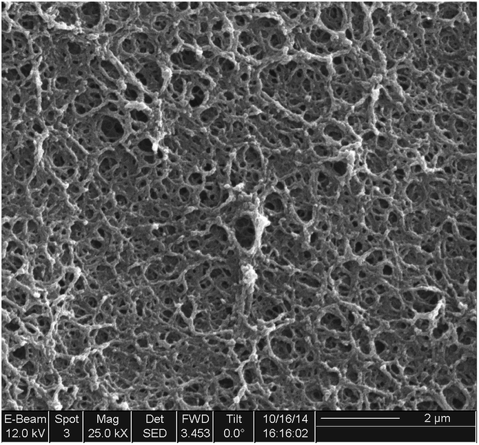 | ||
| Fig. 12 SEM image of porous CS–PEI–GO beads. | ||
4. Conclusions
RSM was a powerful tool to optimize the synthesis of a nanocomposite that can efficiently remove both cationic and anionic metals from water. The composition of the CS–PEI–GO beads were optimized using Box-Behnken Design by varying the concentrations of PEI, GO, and crosslinking agent GLA for maximum removal of Cr(VI) and Cu(II) ions. Second-order polynomial model was adequate to develop the correlation between the independent and dependent variables. ANOVA results show good agreement between experimental and predicted responses, as given by high R2 values of 0.9848 and 0.8327 for Cr(VI) and Cu(II), respectively. Response surface plots revealed the opposite trend of GLA concentration from the responses due to the difference in the mechanisms by which the two metal species are bound to the amine groups of PEI and CS in the nanocomposite. Cr(VI) ions are removed by the adsorbent primarily via electrostatic attraction, while Cu(II) ions form complex structures with the primary amine groups on the surface of the beads. Numerical optimization and validation of the optimized composition of the CS–PEI–GO beads showed good predictability of the model employed for both responses. Lastly, characterization of the optimized beads revealed a chemically and thermally stable material with a mesoporous structure, high surface area and plenty of functional groups present on the surface, all of which are favorable qualities for efficient adsorption capacity. Because of the excellent properties and multi-functionality of the synthesized CS–PEI–GO beads in this study, applicability to other contaminants can be explored, making the new adsorbent very promising for wastewater treatment.Acknowledgements
This project was made possible through the funding from the Texas Hazardous Waste Research Center (THWRC Project Award #: 515UHH0049H), partial funding from the National Science Foundation Career Award (NSF Award #104093), and the Engineering Research and Development for Technology (ERDT) Program of the College of Engineering, University of the Philippines, Diliman.References
- X. Li, Y. Li and Z. Ye, Chem. Eng. J., 2011, 178, 60–68 CrossRef CAS.
- F. Fu and Q. Wang, J. Environ. Manage., 2011, 92, 407–418 CrossRef CAS PubMed.
- Y. Guo, X. Wang, L. Yang, M. Han, J. Zhao and X. Cheng, Environ. Anal. Toxicol., 2012, 2, 154–164 Search PubMed.
- W. Zhang, B. Pan, L. Lv and Q. Zhang, et al., Chem. Eng. J., 2009, 151, 19–29 CrossRef.
- L. Lv, X. Zhao, B. Pan, W. Zhang and S. Zhang, et al., Chem. Eng. J., 2011, 170, 381–394 CrossRef.
- S. C. Smith and D. F. Rodrigues, Carbon, 2015, 91, 122–143 CrossRef CAS.
- I. E. Mejias Carpio, J. D. Mangadlao, H. N. Nguyen, R. C. Advincula and D. F. Rodrigues, Carbon, 2014, 77, 289–301 CrossRef CAS.
- L. Li, L. Fan, M. Sun, H. Qiu, X. Li, H. Duan and C. Luo, Colloids Surf., B, 2013, 107, 76–83 CrossRef CAS PubMed.
- L. Liu, C. Li, C. Bao, Q. Jia, P. Xiao, X. Liu and Q. Zhang, Talanta, 2012, 93, 350–357 CrossRef CAS PubMed.
- Y. L. F. Musico, C. M. Santos, M. L. P. Dalida and D. F. Rodrigues, J. Mater. Chem. A, 2013, 1, 3789 CAS.
- R. L. Tseng, F. C. Wu and R. S. Juang, J. Environ. Manage., 2010, 91, 798–806 CrossRef PubMed.
- W. S. Wan Ngah, L. C. Teong and M. A. K. M. Hanafiah, Carbohydr. Polym., 2011, 83, 1446–1456 CrossRef CAS.
- S. Deng, Environ. Sci. Technol., 2005, 39, 8490–8496 CrossRef CAS PubMed.
- H. N. Lim, N. M. Huang and C. H. Loo, J. Non-Cryst. Solids, 2012, 358, 525–530 CrossRef CAS.
- N. Li and R. Bai, Ind. Eng. Chem. Res., 2005, 44, 6692–6700 CrossRef CAS.
- W. S. W. Ngah and S. Fatinathan, Chem. Eng. J., 2008, 143, 62–72 CrossRef CAS.
- Y. Q. He, N. N. Zhang and X. D. Wang, Chin. Chem. Lett., 2011, 22, 859–862 CrossRef CAS.
- S. H. Wang, H. M. Ang and M. O. Tade, Chem. Eng. J., 2013, 226, 336–347 CrossRef CAS.
- V. M. Boddu, Environ. Sci. Technol., 2003, 37, 4449–4456 CrossRef CAS PubMed.
- R. B. Li Jin, Langmuir, 2002, 18, 9765–9770 CrossRef.
- W. M. Algothmi, N. M. Bandaru, Y. Yu, J. G. Shapter and A. V. Ellis, J. Colloid Interface Sci., 2013, 397, 32–38 CrossRef CAS PubMed.
- C. Y. Yin, M. K. Aroua and W. M. A. W. Daud, Water, Air, Soil Pollut., 2008, 192, 337–348 CrossRef CAS.
- C. Bertagnolli, A. Grishin, T. Vincent and E. Guibal, Ind. Eng. Chem. Res., 2016, 55, 2461–2470 CrossRef CAS.
- D. M. Saad, E. M. Cukrowska and H. Tutu, Water SA, 2013, 39, 257–264 CAS.
- W. Maketon, C. Z. Zenner and K. L. Ogden, Environ. Sci. Technol., 2008, 42, 2124–2129 CrossRef CAS PubMed.
- N. Sui, L. Wang, X. Wu, X. Li, J. Sui, H. Xiao, M. Liu, J. Wan and W. W. Yu, RSC Adv., 2015, 5, 746–752 RSC.
- L. G. Chen Fei, Y. Weiwei and W. Yujun, Tsinghua Sci. Technol., 2005, 10, 535–541 CrossRef.
- B. Qiu, J. Guo, X. Zhang, D. Sun, H. Gu, Q. Wang, H. Wang, X. Wang, X. Zhang, B. L. Weeks, Z. Guo and S. Wei, ACS Appl. Mater. Interfaces, 2014, 6, 19816–19824 CAS.
- P. Yin, Z. Wang, R. Qu, X. Liu, J. Zhang and Q. Xu, J. Agric. Food Chem., 2012, 60, 11664–11674 CrossRef CAS PubMed.
- G. Wang, S. Zhang, T. Li, X. Xu, Q. Zhong, Y. Chen, O. Deng and Y. Li, RSC Adv., 2015, 5, 58010–58018 RSC.
- A. Long, H. Zhang and Y. Lei, Sep. Purif. Technol., 2013, 118, 612–619 CrossRef CAS.
- D. C. Marcano, D. V. Kosynkin, J. M. Berlin, A. Sinitskii, Z. Sun, A. Slesarev, L. B. Alemany, W. Lu and J. M. Tour, ACS Nano, 2010, 4, 4806–4814 CrossRef CAS PubMed.
- J. Qi and W.-C. Shih, Appl. Opt., 2014, 53, 2881–2885 CrossRef CAS PubMed.
- H. Zhu, Y. Fu, R. Jiang, J. Yao, L. Xiao and G. Zeng, Ind. Eng. Chem. Res., 2014, 53, 4059–4066 CrossRef CAS.
- H. Wang, X. Yuan, Y. Wu, H. Huang, G. Zeng, Y. Liu, X. Wang, N. Lin and Y. Qi, Appl. Surf. Sci., 2013, 279, 432–440 CrossRef CAS.
- X. Li, H. Zhou, W. Wu, S. Wei, Y. Xu and Y. Kuang, J. Colloid Interface Sci., 2015, 448, 389–397 CrossRef CAS PubMed.
- Z. Bo, X. Shuai, S. Mao, H. Yang, J. Qian, J. Chen, J. Yan and K. Cen, Sci. Rep., 2014, 4, 4684 Search PubMed.
- M. N. Parul Rana-Madaria, C. Rajagopal and B. S. Garg, Ind. Eng. Chem. Res., 2005, 44, 6549–6559 CrossRef.
- K. K. Jyotsna Goel, C. Rajagopal and V. K. Garg, Ind. Eng. Chem. Res., 2005, 44, 1987–1994 CrossRef.
- A. A. R. A. Igder and A. Fazvali, et al., Int. J. Min., Reclam. Environ., 2012, 3, 51–59 Search PubMed.
- M. Sarkar and P. Majumdar, Chem. Eng. J., 2011, 175, 376–387 CrossRef CAS.
- F. Shakeel, N. Haq, F. K. Alanazi and I. A. Alsarra, Ind. Eng. Chem. Res., 2014, 53, 1179–1188 CrossRef CAS.
- W. Zhang, Z. Zhu, M. Y. Jaffrin and L. Ding, Ind. Eng. Chem. Res., 2014, 53, 7176–7185 CrossRef CAS.
- C. J. Luk, J. Yip and C. M. Yuen, J. Fiber Bioeng. Informat., 2014, 7, 35–52 Search PubMed.
- M. Amara and H. Kerdjoudj, Talanta, 2003, 60, 991–1001 CrossRef CAS PubMed.
- I. D. Migneault, C. Dartiguenave, M. J. Bertrand and K. C. Waldron, BioTechniques, 2004, 37, 798–802 Search PubMed.
- Y.-J. Jiang, X.-Y. Yu, T. Luo, Y. Jia, J.-H. Liu and X.-J. Huang, J. Chem. Eng. Data, 2013, 58, 3142–3149 CrossRef CAS.
- L. Fan, C. Luo, M. Sun, X. Li, F. Lu and H. Qiu, Bioresour. Technol., 2012, 114, 703–706 CrossRef CAS PubMed.
- D. Han, L. Yan, W. Chen and W. Li, Carbohydr. Polym., 2011, 83, 653–658 CrossRef CAS.
- O. A. C. Monteiro Jr and C. Airoldi, Int. J. Biol. Macromol., 1999, 26, 119–128 CrossRef CAS.
- L. Yang, B. Tang and P. Wu, J. Mater. Chem. A, 2014, 2, 18562–18573 CAS.
- Q. Zhang, J. Teng, G. Zou, Q. Peng, Q. Du, T. Jiao and J. Xiang, Nanoscale, 2016, 8, 7085–7093 RSC.
- Q. Zhang, Q. Du, M. Hua, T. Jiao, F. Gao and B. Pan, Environ. Sci. Technol., 2013, 47, 6536–6544 CAS.
- H. Qiu, C. Liang, J. Yu, Q. Zhang, M. Song and F. Chen, Chem. Eng. J., 2017, 315, 345–354 CrossRef CAS.
Footnote |
| † Electronic supplementary information (ESI) available. See DOI: 10.1039/c7ra00750g |
| This journal is © The Royal Society of Chemistry 2017 |