Development of small-volume, microfluidic chaotic mixers for future application in two-dimensional liquid chromatography

Abstract

We report a microfluidic chaotic micromixer with staggered herringbone grooves having a geometry optimized for fast mobile-phase modification at the interface of a two-dimensional liquid chromatography system. The volume of the 300 μm mixers is 1.6 microliters and they provide mixing within 26 s at a flow rate of 4 μL min⁻¹ and 0.09 s at a flow rate of 1000 μL min⁻¹. Complete mixing is achieved within a distance of 3 cm along the 5 cm-long microchannel over the whole range of flow rates. The mixers can be used to mix aqueous phosphate-buffered saline solutions with methanol or acetonitrile at different ratios (1 : 2, 1 : 5 and 1 : 10). We also describe in detail an improved fabrication protocol for these mixers using a two-step soft photolithographic procedure. Mixers are made by replication in poly(dimethylsiloxane).

---

1 Introduction

The increasing demand for analysis of more complex samples is stimulating the development of high-resolution multidimensional separation techniques, such as two-dimensional (2D) liquid chromatography (LC).^1,2 Coupling different separation mechanisms in 2D LC has two important consequences. First, as the separation mechanism in LC is determined by the nature of stationary and mobile phases, coupling two columns (two dimensions) with different stationary phases necessarily means that each dimension requires a different mobile phase. This leads to a major issue in 2D LC, namely how to deal with solvent incompatibility between dimensions. This often means that a solvent in the first dimension (¹D) becomes a strong eluent in the second dimension (²D), rapidly eluting analytes. This results in so-called breakthrough on the second column, and poor separation of analytes as a result. Additionally, viscosity differences and immiscibility of solvents can cause flow instability (viscous fingering effect) in situations where mobile phases of mixed composition are required (e.g. gradient elution). This can lead to distortion of the peak shape in the second dimension.³

The second consequence of coupling two columns is the requirement of a specially designed interface to maintain the resolution of the separation in the first dimension for the second dimension separation. It should provide for the efficient fast transfer of ¹D effluent to the ²D and allow modification of the solvent composition between dimensions. The interface usually consists of a 10-port valve with either two loops for cutting ¹D effluent into small fractions⁴ or trap-columns for pre-concentration of analytes before re-injection onto the second column,⁵ or both.⁶

A dilution of the ¹D effluent with ²D mobile phase improves the sample focusing in the ²D which is crucial for overall good performance of 2D LC. For the purpose of solvent modification between dimensions, an additional pump and a mixer unit are required. As such a dilution can lead to peak broadening, the mixer should have a small internal volume (low-μL range) to obtain the desired dilution ratios in minimal volumes. Additionally, the small volume of the mixer should enable fast modification (20–30 s) and maintain small sampled portions of ¹D effluent. The most used mixing unit in the area of LC nowadays is the T-piece, in which two streams are simply collided with each other, with optimal mixing obtained at higher flow rates. Another commercially available mixer for LC applications is the so-called static mixer (S-mixer, e.g. HyperShear™ HPLC).⁷ S-Mixers are usually composed of two periodically repeated elements in the axial direction. Each element consists of two pairs of four crossed bars perpendicular to the orientation of the fluid stream.⁸ Thus, the fluid interface experiences stretching and folding eight times while moving through each element. The mixing efficiency of the S-mixer improves with higher flow rates and bigger volumes,⁷ making it inherently unsuitable for 2D LC purposes. In order to obtain mixing in small volumes and over a wide range of flow rates, we propose to use chip-based microfluidic technologies,⁹ which focus on the development of tools for manipulation of small volumes of fluids. Perhaps the best example of attempts to implement microfluidic technologies in an LC system is the commercially available Jet Weaver mixer.¹⁰ This device employs a network of multi-layer microfluidic channels (120 μm × 120 μm), and uses the split-and-recombine principle to ensure efficient solvent gradient formation. It is incorporated into the HPLC pumping system (1290 Infinity Binary pump) and is available in volumes of 35 μL, 100 μL and 380 μL. Our mixer differs substantially from this device, as it has a much smaller internal volume and is based on chaotic mixing, which ensures fast mixing in small volumes over a wide range of flow rates.

Mixing at the micrometer scale is a challenge because of the existence of well-defined laminar flow under typical flow conditions in microchannels. A number of approaches to overcome this limitation have been proposed, including passive and active micromixers that can rapidly mix small amounts of fluids.^11–13 Passive micromixers are generally preferred since they are easier to fabricate and do not require the application of an external force to achieve mixing, which makes them more robust and stable. The approach chosen for this work was first described by Stroock et al.¹⁴ and is based on passive chaotic mixing. Mixing is achieved through the incorporation of microgrooves into a microchannel wall. Grooves can be positioned in arrays at an oblique angle to the wall (slanted grooves, SG), or take the shape of asymmetric chevrons or herringbones in staggered arrays (herringbone grooves, HG). These grooves work as obstacles placed in the path of the flow and alter the laminar flow profile. This leads to a dramatic increase of the contact area between the two streams, and facilitates mixing by diffusion. Herringbone grooves generate two counter-rotating vortices (perpendicular to the direction of the flow) whereas slanted grooves create a helical or corkscrew pattern flow.¹⁴

Chaotic mixers with embedded microgrooves have been found to work well for systems with Reynolds numbers from 1 to 100.¹⁴ Several studies report the utilization of mixers to improve a surface electrochemical reaction,^15,16 perform on-line chemical modification of peptides,¹⁷ and provide mixing for direct and sandwich immunoassays.¹⁸ There are other alternative applications in the area of surface interactions, such as binding of DNA on magnetic beads;¹⁹ focusing, guiding and sorting particles;²⁰ and the binding of proteins²¹ and circulating tumor cells to functionalized surfaces.^22,23 Most of these applications utilize the same dimensions of the mixer reported in the original study,¹⁴ not altering them to better satisfy the demands of the current application or optimizing them based on numerical computational studies available in the literature. This often leads to the implementation of non-optimal micromixer designs and suboptimal performance.

The aim of this work was to develop a chaotic mixer for fast mixing performance in a given small volume for future application in 2D LC for solvent modification between columns. For this, we used an approach taken from the literature to design optimized grooved microfluidic mixers with internal volumes on the order of just 1 or 2 microliters. We also characterized the mixer in order to ensure its applicability to the 2D LC system. We demonstrated the possibility of using small-volume micromixers for flow rates compatible with 2D LC (300–1000 μL min⁻¹). Also, devices were tested for mixing solutions with different compositions and viscosities, such as phosphate-buffered saline/acetonitrile and phosphate-buffered saline/methanol mixtures, which are the most common solvents used in liquid chromatography. In addition, the fabrication process of mixers is described in detail. We believe that our approach represents one further step in the implementation of microfluidic technologies for mixing in conventional LC.

2 Materials and methods

Information regarding chemicals and reagents can be found in the ESI.†

2.1 Mixer parameters and optimization

The mixer has a Y-shaped channel with two inlets and one outlet (Fig. 1A). The mixing channels are 50 mm long (from the Y-junction) and 300 or 400 μm wide. A ruler is located along the channel to show the distance from the Y-junction. The total volume of the mixing channel is about 1.6 μL and 2.2 μL for widths of 300 and 400 μm, respectively.

Fig. 1 (A) Photograph of the poly(dimethylsiloxane) (PDMS) – glass chip with tubing inserted into inlets and outlet. The total channel length is 50 mm. (B) Schematic drawing of grooves in a channel: h – channel height; d – groove depth; a – groove width; b – groove spacing; θ – groove intersection angle. Schematic drawing of the channel top-view illustrating (C) two full cycles in channel with HG; (D) channel with SG. Inlet channel dimensions: 5.2 mm long and 150 μm wide for 300 μm-wide channels, and 6 mm long and 200 μm wide for 400 μm-wide channels.

The geometry of the grooves is determined by their depth (d), width (a) and groove spacing (b) (Fig. 1B). These parameters are the same for the HG and SG tested. Additional parameters for the HG are the asymmetry index, p, between long and short groove arms (p is the fraction of channel width occupied by the long arm of a HG i.e. p = w_l/w) and groove intersection angle (θ). The groove depth-to-channel height ratio (d/h) (hereafter known as “groove-depth ratio”) for both slanted and herringbone grooves and p were found to have the greatest influence on mixing efficiency.²⁴

All geometric ratios – groove-depth ratio (d/h), groove spacing-to-channel width ratio (b/w) and channel-aspect ratio (h/w) – were found to be interdependent, and there exists an optimal groove width-to-channel width ratio (a/w) that maximizes mixing efficiency.²⁵ Table 1 compares optimal channel and groove parameter values taken from the literature that maximize mixing efficiency²⁵ with measured values of these parameters for fabricated devices (actual parameters).

Table 1 Optimal channel and groove parameter values taken from the literature that maximize mixing efficiency²⁵ compared with measured values of these parameters for fabricated devices (actual parameters)

Channel parameters	Optimal (based on^25)	Channel 1	Channel 2
w – channel width (chosen), μm	300/400	300	400
h/w – channel aspect ratio	0.2/0.15	0.2	0.15
h – channel height, μm	60	60	60
d/h – groove depth to channel height ratio	≥1.6	0.8	0.8
d – groove depth, μm	96	50	50
p – asymmetry index	0.58–0.67	0.62	0.62
θ – groove intersection angle, °	90	90	90
a – groove width, μm	120/160	105 ± 5	120 ± 2
b – groove spacing, μm	45/60	50 ± 2	65 ± 2
n – number of grooves per half cycle	5–6	6	6

---

One of the most important parameters for mixer design is the groove depth ratio (d/h). Previous studies^24,25 showed that mixing performance of both slanted and herringbone grooves improves with an increase in the value of d/h, achieved using deeper grooves with respect to channel height. This can be explained by the increased fluid entrainment in the grooves leading to an increase of the vertical motions of the fluid at the side edges of the groove.²⁶ The influence of d/h on mixing was investigated experimentally; channel heights were varied from 60 to 90 μm while groove depths were varied from 50 to 20 μm deep, respectively, to achieved d/h of 0.83 down to 0.22. Results will be discussed in Section 3.1. Note that the optimal d/h is 1.6 for a given h/w, according to Lynn and Dandy. This would lead to a groove depth of 96 μm, which could pose problems from a fabrication perspective as well as introduce excessive dead volume, adversively affecting chromatographic performance.

Another important parameter is the groove asymmetry (p). The effect of p on the mixing performance was investigated by Li and Chen using the lattice-Boltzmann method for computational simulation and optimization of chaotic micromixers based on particle mesoscopic kinetic equations.²⁷ The long groove arm is believed to transport fluid to the other side of the channel. The stirring effect generated in this way is increased through the interchange of the positions of short and long groove arms every half cycle (Fig. 1C). Such alteration of the flow motion causes a change in the position of asymmetric vortices that appear in each half cycle.²⁸ The optimal value of p was found to be 0.6.²⁷ The same result was shown by Lynn and Dandy,²⁵ and Stroock.¹⁴

Several groups have studied the effect of the number of grooves per half cycle (n) on the mixing performance. Li and Chen found that the mixing depends on n as long as n ≥ 4.²⁷ The optimal number of grooves per half cycle was found to be 5–6 grooves.²⁷ Another study showed that more mixing cycles lead to better mixing efficiency than more grooves per cycle.²⁹ Also, previous experiments reported by Stroock^14,30 showed that grooves with an oblique angle of 45° (SG) and an intersection angle of 90° (HG) can generate maximum transverse flows.

Lynn and Dandy showed for SG that wider grooves (larger a) with smaller groove spacing (smaller b) increase of the magnitude of secondary flow by up to 50% compared to the case where a = b.²⁵ However, increasing the width of the groove will result in more pronounced helical motion only to some extent. According to Du et al.,³¹ the mixing length (the distance along the channel at which two solutions are well mixed) decreases sharply as a/w is increased from 0.2 to 0.25. However, the mixing performance is hardly improved when the a/w is further increased to 0.4. Decreasing the groove spacing also allows an increase in the number of cycles within the same channel length.

2.2 Chip fabrication and assembly

The microchannels were constructed by standard microfabrication and replicated in the silicone rubber, poly(dimethylsiloxane) (PDMS) (Sylgard 184, Dow Corning, U.S.). The PDMS channels were sealed by bonding to glass. The chip layout and design were drawn using the software Clewin (Wieweb software, Hengelo, The Netherlands). SU-8 masters were fabricated in a similar way to that used by Stroock,¹⁴ through two steps of standard photolithography. To the best of our knowledge, no detailed description of the fabrication has been presented in the literature, though a number of papers refer generally to the fact that two-step photolithography is used. We therefore present a more detailed description of the process used to fabricate the masters in the ESI.†

Grooved microchannels were fabricated by casting a solution of PDMS prepolymer onto the master. PDMS resin and curing agent were mixed at a weight ratio of 10 : 1 and manually stirred to mix thoroughly. The stirred solution was exposed to mild vacuum for 30 min to remove air bubbles. After curing on a hot plate for an hour at 70 °C, the PDMS layer was cut into individual devices and peeled off the master (there were two devices on one wafer).

Holes were punched (1.5 mm (od)) into the PDMS device at the locations of the inlets and outlet, and the glass slides were cleaned with acetone and 96% ethanol. In order to bond the PDMS channel to the glass slide, PDMS chips and glass slides were exposed to oxygen plasma for 20 s. Afterwards, the treated surfaces were immediately brought into contact with each other. The assembled chips were placed on a hot plate for 30 min at 70 °C to enhance the formation of a chemical bond, after which chips were taken from the hotplate to cool down to room temperature. Teflon tubing (0.8 mm (id), 1.6 mm (od), Polyfluor Plastics, The Netherlands) was inserted directly into the punched holes in the PDMS layer (Fig. 1A).

2.3 Experimental setup

In order to characterize the degree of mixing, fluorescence detection was used. Fluorescein (5 μM) in phosphate buffer and phosphate buffer were introduced from separate inlets into the Y-junction of the channel at different flow rates using syringe pumps with 5 mL syringes (Prosense, The Netherlands).

The Péclet number (Pe) was used to calculate the flow rates required in channels with different widths to perform experiments under the same conditions of molecular mass transport. The Péclet number is a dimensionless parameter that characterizes molecular mass transport in flow conduits as a ratio of advective transport (flow) rate to diffusive transport rate:

Here v is the average linear velocity (mm s⁻¹) and D represents the diffusion coefficient (mm² s⁻¹); d_h denotes the hydraulic diameter for a rectangular duct (e.g. equivalent diameter of a channel, mm):where h is channel height (mm), d, groove depth (mm), and w, channel width.

Mixing was then tested under constant Péclet-number conditions rather than constant flow rates to ensure the same mass transport conditions in devices with different dimensions (Table 2).

Table 2 Tested flow rates based on Péclet-number calculation for channels with different widths; d + h = 110 μm; d_h = 0.161 mm (w = 300 μm), d_h = 0.173 mm (w = 400 μm), ρ = 10³ kg m⁻³, μ = 10⁻³ kg (m s)⁻¹, D = 2.6 × 10⁻¹⁰ m² s⁻¹ (for fluorescein)³²

Pe, 10^3	Channel width, μm		Re
	300	400
	Total flow rate, μL min^−1	Total flow rate, μL min^−1
1.0	3.7	4.6	0.3
10.0	37	46	3.0
30.0	111.0	138.0	9.0
50	185.0	230.0	15.0
100	370.0	460.0	30.1
150	556.0	691.6	45.2
200	740.0	920.5	60.1
300	1112.5	1383.2	90.4

---

The Reynolds number (Re) was also calculated in order to confirm that laminar flow conditions were used for experiments. Re is a dimensionless number that gives a measure of the ratio of inertial forces to viscous forces for given flow conditions:

where d_h denotes relevant length (see eqn (2)), v is average linear velocity (m s⁻¹), ρ equals the density of the fluid (kg m⁻³) and μ represents the dynamic viscosity of the fluid (kg (m s)⁻¹). All experiments were performed under laminar flow conditions (Re ≪ 2000).

The chip was placed under a fluorescent microscope (model “DMIL”, Leica Microsystems, The Netherlands), equipped with a 4× objective, an external light source for fluorescence (EL6000, Leica Microsystems, The Netherlands), and a CCD camera. For visualization of fluorescence, a fluorescein filter set (488 nm excitation, 518 nm emission) was used. Images were captured at different positions along the channel with a CCD camera connected to a computer using a 4× objective magnification with a field of view of 1.8 mm, a 1 s exposure time, a gamma setting of 1.75, and a gain of 3.5.

To investigate the mixing mechanism and monitor the mixing behavior over the cross-sections of the mixing channel, we utilized a confocal microscope (LEICA TCS SP8, Leica Microsystems B.V.). Devices were mounted on the moving microscope stage and syringes from syringe pumps were connected to the inlets of the devices. More information about these experiments may be found in the ESI,† Section 3.

All experiments were performed in triplicate using different chips from different masters which were fabricated using the same procedure.

2.4 Data analysis

The degree of mixing was quantified by determining the standard deviation (SD) in fluorescence intensity across the width of the channel at different locations along its length. The SD was calculated using the following eqn (4):³³Here, x_i is the gray-scale intensity value of pixel i, and x̄ is the mean intensity value of pixels across the entire channel. In order to be able to compare different parts of the channel, normalized fluorescent intensity was used:

For this, SD (eqn (4)) was normalized by the total intensity value of pixels across the channel (x_i). In order to compare different chips, the value of SD_norm for the position 0 mm was set as 0.5, and the SD values for the other positions were calculated respectively. A normalized SD of 0 represents completely mixed solutions (when the intensity is uniform across the channel), whereas a value of 0.5 indicates unmixed solutions.

To calculate SD, images were analyzed using LispixLx85P free software (Allegro Common LISP v. 8.0, (c) 2004 Franz Inc.) by determining the SD of the intensity distribution across the width of the channel. It should be mentioned that a SD value of 0.01, which corresponds to 98% mixing, can be considered as corresponding to a completely mixed situation, as introduction of premixed solutions in the channel yields a SD value of 0.01. Thus, SD cannot reach a value of 0. This relates to the uniformity of pixel intensity values on the image itself captured by the CCD camera. We define mixing efficiency as the ability to accomplish mixing with a minimum time and length. Mixing within 20–25 mm of the channel is efficient. We consider 98% (SD 0.01) as corresponding to complete mixing.

3 Results and discussion

3.1 Optimization of mixing channel design

For application in the 2D LC interfaces, it is important that the passive chaotic micromixers under consideration possess small internal volumes (on the order of just a few μL). At the same time, these components should not contribute significantly to overall pressure drops in the system at the flow rates typically used in ¹D (100's of μL per minute). Hence, we chose for devices having internal volumes of 1.6 μL and 2.2 μL (1.5 to 2 times larger than those reported by Stroock et al.¹⁴) with total channel length of 50 mm in order to maintain pressure drops below 1 bar.¹⁴ However, the dimensions used by Stroock et al.¹⁴ cannot simply be multiplied by a constant to achieve mixers with bigger volumes exhibiting the same performance (mixing efficiency). Particularly important is the selection of groove depth, width and spacing in relation to altered channel widths and depths. Optimized channel and groove parameters used in this study for SG and HG mixers (Table 1) were thus selected or calculated based on a previously described numerical study by Lynn and Dandy.²⁵

In order to increase the inner volume of the mixer with respect to the original report by Stroock et al.,¹⁴ microchannels having widths, w, of 300 and 400 μm and a height, h, of 60 μm were used for this study. After choosing the values of w and h to establish channel aspect ratios, h/w, of 0.20 (w = 300 μm) or 0.15 (w = 400 μm), other groove parameters (groove depth, d; groove width, a; and groove spacing, b) were selected or calculated based on h/w (Table 1).²⁵ θ, n and p were kept constant in this study; d/h, h/w, a/w and b/w were varied.

To test the influence of d/h on mixing, microchannels with HG having different h and d were fabricated. Three different HG mixers were realized, with d/h = 0.22 (d = 20 μm, h = 90 μm), d/h = 0.37 (d = 30 μm, h = 80 μm), and d/h = 0.83 (d = 50 μm, h = 60 μm). The results obtained are shown in Fig. 2, where a definite increase in mixing efficiency is observed as d/h is increased. SD decreased (mixing efficiency increased) as a function of channel length.

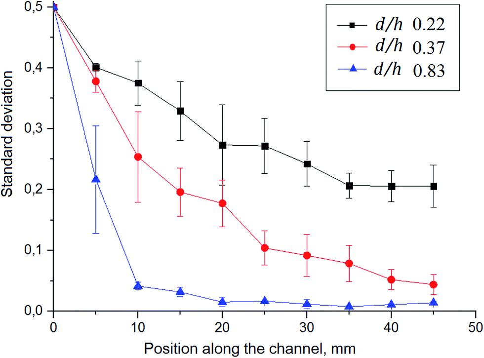Fig. 2 Influence of the groove depth-to-channel height ratio, d/h, on mixing performance in an HG mixer (n = 3 chips). The total flow rate is 20 μL min⁻¹; 300 μm-wide channel; fluorescein (5 μM) in PBS was mixed with PBS in a 1 : 1 flow rate ratio; total channel length is 50 mm. The variations in standard deviation are due in part to the fact that these experiments were carried out over a period of several months, during which time the lab environment varied somewhat and final adjustments to the fabrication protocol were being made.

For d/h= 0.83 in Fig. 2, complete mixing has been essentially achieved at a channel length of 20 mm from the Y-junction. In contrast, mixing has only been partially achieved at 20 mm for d/h = 0.22 and 0.37. This is consistent with observations made in other studies.^14,25,26 A probable explanation is related to the two counter-rotating vortices generated in HG mixers. The size of the larger vortex, formed above the longer arms of the herringbone grooves, grows as d/h increases.³⁴ (Section S3 of the ESI† shows confocal microscopic images of the cross-sectional flow profile recorded along the length of a HG mixer with w = 300 μm.) Thus, deeper grooves provide an enhancement in mixing. However, Du et al.³¹ showed that increasing the d/h-value is only effective for enhancing mixing within a limited range of d/h. Optimum values of d/h may be found in a range of 0.28 to 0.7 if h is decreased or for d/h values between 0.25 and 0.4 if d is increased. A further increase in d in this latter case does not lead to faster mixing. This can be explained by considering the location of the transverse fluid transport caused by grooves. In the microchannel, mixing occurs above the grooves where the vortices are to be found, and chaotic mixing proceeds rapidly as a result. Mixing also occurs within the grooves; however, mixing in this region is much less rapid, as it is dictated by laminar flows and slow diffusion. When d is increased, a large quantity of fluid (more than 60%) enters the grooves, and the slow diffusional mixing inside the groove becomes significant with respect to the overall mixing inside the channel.³¹ A deeper groove could result in a bigger dead volume, in which molecules could be retained for inordinately long periods of time in real applications, making mixing inefficient.²⁷

The optimal d/h value for the chosen h/w ratios was 1.6 or larger, according to Lynn and Dandy.²⁵ However, for h = 60 μm, this implies grooves that are at least 96 μm deep. This would introduce a large dead volume to the mixer which could adversely influence chromatographic results through increased band broadening in future applications. For this reason, d/h = 0.8 was chosen (d = 50 μm h = 60 μm). This value still provides enhanced mixing, but does not contribute a large dead volume as discussed below.

3.2 Mixing performance in the different types of microchannels with different groove arrays

In order to determine which mixer exhibits the most suitable performance for the application at hand, three types of microchannels were investigated: (1) channels with slanted grooves (SG) and (2) herringbone grooves (HG), and (3) channels with no grooves (NG). In addition, channels having w = 300 μm or 400 μm were studied. The efficiency with which PBS and PBS-fluorescein solutions are mixed in these types of channels is compared in Fig. 3. The standard deviation of fluorescence intensity across the channel is plotted versus distance along the channel for a wide range of flow rates. Experiments were carried out in channels with w = 300 μm (Fig. 3A) and w = 400 μm (Fig. 3B) in the range of Pe values from 10³ to 3 × 10⁵ (Table 2). Data is shown only for low (Pe = 10³, solid line) and high (Pe = 10⁵, dashed line) flow rates in Fig. 3.

Fig. 3 Comparison of microfluidic mixers having no grooves (NG), slanted grooves (SG) and herringbone grooves (HG) as a function of distance from the Y-junction for channel widths of 300 μm (A) and 400 μm (B) at different flow rates: Pe = 10³ (solid line) and Pe = 10⁵ (dashed line). The flow rate in each case is the total flow rate in the mixing channel, with a 1 : 1 flow rate ratio of PBS (fluorescein)–PBS; n = 3 chips. For grooved channels: d = 50 μm and h = 60 μm; for channels with no grooves , h = 110 μm; a = 105 μm for the 300 μm-wide channel, a = 120 μm for the 400 μm-wide channel. (C) Standard deviation versus position along the channel for the 300 μm-wide HG mixer for Pe in the range of 10³ to 3 × 10⁵, which corresponds to the flow-rate range of 3.7 to 1114 μL min⁻¹ (Table 2). Photographs are presented to show mixing at (a) 0 mm; (b) 5 mm; (c) 15 mm; (d) 35 mm. (D) Residence times at different flow rates (Pe = 10³ to 10⁵) for HG mixer; flow-rate ratio of PBS (fluorescein)–PBS was 1 : 1; total channel length is 50 mm for all channels. The observed range of standard deviation is 0.05–0.15 at 5 mm.

Incomplete mixing is observed in the NG channel at low flow rate (Pe = 10³) at a channel length of 50 mm for both channel widths studied. The mixing in these channels relies entirely on diffusion of molecules between side-by-side flows, which is a slow process. (Molecules would require more than 10 seconds to diffuse from the interface between solution streams at the middle of the channel to the sides. This is a long time when compared to the residence time of molecules in the channel at even low flow rates, see Table 2 and Fig. 3D.) In fact, mixing at the lower flow rate in the 300 μm-wide channel with no grooves (NG) (Fig. 3A), though incomplete at the end of the 50 mm channel, is more complete than in the 400 μm-wide channel with no grooves (NG) (Fig. 3B). This is in keeping with the longer radial distance that solutes need to travel by diffusion for mixing to occur in the wider channel.

Increasing the flow rate by a factor of 100 (Pe = 10⁵) would lead to decreased residence times of solutes in the microchannel and thus to negligible mixing or no mixing at all. Introducing a mixer with slanted or herringbone grooves results in more efficient mixing, as presented in Stroock's original study.¹⁴

For the grooved channels, we observe a similar decrease in mixing efficiency, especially at low flow-rate, for the 400 μm-wide channel compared to the 300 μm-wide channel, which means that, perhaps, similar diffusional effects as discussed above could still be playing a role. We tried to compensate for the increase in w/h by maintaining the a/w ratio, widening the grooves from 105 μm (as in the 300 μm-wide channel in Fig. 3A) to 120 μm for the 400 μm-wide channel in Fig. 3B. Based on experimental data which is not shown, we assume that even wider and deeper grooves would improve the mixing efficiency further in the 400 μm-wide channel. Considering the better performance of the 300 μm-wide channel (Fig. 3A and B) and its smaller volume (1.6 μL compared to 2.2 μL of the 400 μm-wide channel), we selected the 300 μm-wide channel for further studies.

If we look at channels which are 300 μm wide, it can be seen that in the HG mixer (red dots on Fig. 3A), 98% of mixing is completed by a distance of 10 mm and 15 mm for Pe of 10³ and 10⁵, respectively. These findings are in good agreement with values obtained by Stroock¹⁴ for the same Péclet number but for a channel with smaller cross-sectional area. For the SG mixer (blue dots, Fig. 3A), the required distances for complete mixing are 20 and 35 mm for Pe of 10³ and 10⁵, respectively. From these data, we can conclude that herringbone grooves provide better mixing performance than slanted grooves for all the flow rates tested. This is consistent with observations from other studies.^25,35 The HG mixer is 30 and 55 times more efficient than the NG channel, and 2.0 and 3.8 times more efficient than the SG mixer, at 3.7 μL min⁻¹ and 370 μL min⁻¹, respectively (at a channel position of 45 mm in Fig. 3A). The reason for the better efficiency of the HG mixer lies in the difference between the processes involved in mixing. In general, grooves enhance mixing because of the additional motion of fluids (stretching and folding), which leads to an increased contact area between the solutions to be mixed, thereby decreasing diffusion lengths. Stretching and folding of solution volumes inside the mixers proceeds exponentially as a function of the distance travelled along the channel.^14,36 In the SG mixer, mixing happens through generation of a single helical flow along the axis of flow (a more detailed mechanism for SG is reported elsewhere).³⁷ This requires a longer distance to complete mixing. In contrast, mixing in the HG mixer occurs as a result of the formation of two oppositely rotating vortices across the channel. This makes the HG mixer more efficient.

In order to investigate the influence of Péclet number on mixing efficiency, we tested the 300 μm-wide HG mixer over a wide range of Péclet numbers, namely 10³ to 3 × 10⁵ which corresponds to a flow-rate range of 3.7 to 1114 μL min⁻¹ (Table 2). As seen in Fig. 3C, the HG mixer performed well over the whole chosen range of Pe. Initially, the intensity decreased sharply (decrease in SD, Fig. 3C(a) and (b)) within the first 10 mm of channel length and then quickly leveled off to approach a constant value, which corresponded to complete mixing. As expected, the efficiency of mixing decreased with an increase of the flow rate, but only over the first 15 mm of the channel. The observed SD varies from about 0.25 to about 0.05 at 5 mm for flow rates from 1114 to 3.7 μL min⁻¹, whereas it varies from 0.01 to 0.008 at 40 mm for the same flow-rate range in this 300 μm-wide HG channel. Complete mixing was achieved by 15 mm, independent of the flow rate. This can be explained by the compensation of shorter residence (and diffusion) times by increased agitation of the flows, which leads to more chaotic flow patterns. Such effects make the HG mixer efficient over a wide range of flow rates. The observed variation in fluorescence intensity was the same as in Stroock's study,¹⁴ who concluded that the form of the flow remains qualitatively the same for 0 < Re < 100 (Pe > 10⁶).

As Pe increases by a factor of 300 (from 10³ to 3 × 10⁵), the distance required for 98% mixing (SD = 0.01) increases by a factor of 1.5 (from 10 mm to 15 mm). Complete mixing requires a relatively longer distance (additional 5–10 mm) at higher flow rate (Pe ≥ 10³). Shorter residence times, leading to shorter diffusion times, account for this observation, as already alluded to above (Fig. 3D). Residence time (R_t, s) was calculated as the centre-line length of the channel (cm) divided by the average flow velocity (cm s⁻¹). The calculated values of R_t underline the speed of mixing, particularly at higher flow rates. As seen from Fig. 3D, mixing can be achieved in the 300-μm-wide channel within a distance of 20 mm in 10.7 s, 1.1 s and 0.11 s at total flow rate 3.7 μL min⁻¹ (Pe = 10³), 37 μL min⁻¹ (Pe = 10⁴) and 370 μL min⁻¹ (Pe = 10⁵), respectively. With herringbone grooves, then, the increased flow rate leads to almost the same mixing distance but in a much shorter period of time, which is beneficial for fast solvent modification in 2D LC. Also, it is clear that potential dead volumes in the grooves themselves is not an issue.

3.3 Mixing of different solvents

Micromixers designed in this study will be implemented for the modification of mobile phase eluting from the first dimension before entering the second dimension in 2D LC. This application requires mixing of different solvents to tune the ability of a mobile phase to elute analytes from a stationary phase. In order to investigate the efficiency of the HG mixer, two of the most commonly used solvents in liquid chromatography, acetonitrile (ACN) and methanol (MeOH), were chosen for further experiments. First, these solvents were mixed with phosphate-buffered saline (PBS) at equal (1 : 1) flow-rate ratios. Fig. 4 shows images obtained with a fluorescent microscope which have been stitched together to show the first 20 mm of the 300 μm-wide, 60 μm-deep channel with herringbone grooves (d = 50 μm). The solution of fluorescein in PBS (green color) from the left inlet (upper inlet in images) and solution of PBS (Fig. 4A), ACN (Fig. 4B) or MeOH (Fig. 4C) from the right inlet (lower inlet in images) were introduced at equal flow rates. As the mixing proceeds along the channel, the observed fluorescence gradually expands to cover the whole channel width, and an almost equal distribution of fluorescence can be observed at the 20 mm mark in the channel, indicating almost complete mixing. Here, as in all previous experiments, the absolute intensity of the fluorescence decreases, which is related to the dilution effect. The same chaotic flow patterns, observed with confocal microscopy in the channel cross-section (ESI, Fig. S2†), appear as striations when viewed from above in Fig. 4.

Fig. 4 Fluorescence images taken from above of HG micromixers in which a solution of fluorescein in PBS is mixed with (A) PBS solution, (B) ACN, (C) MeOH at a 1 : 1 flow-rate ratio; images have been stitched together to show the first 20 mm of the 300 μm-wide channel, Pe = 2.7 × 10⁵, Re = 81 (same channel used in Fig. 3).

In order to enable the solvent modification between dimensions in 2D LC, a relevant solvent (e.g. water) should be mixed with the ¹D effluent. In most cases, the ¹D effluent will contain a high percentage of organic solvent which should be diluted five or ten times. Thus, ACN or MeOH were introduced together with PBS solution at different flow-rate ratios: 1 : 1, 1 : 2, 1 : 5 and 1 : 10 (Fig. 5). A solution of 5 μM fluorescein in PBS was used to visualize the mixing. All experiments were designed to maintain a total flow rate of 1 mL min⁻¹ (Pe = 2.7 × 10⁵). In general, for both ACN/PBS and MeOH/PBS systems, no significant difference in mixing efficiency was observed and the mixing was complete at a distance of 45 mm. The fact that mixing efficiency was unaffected by buffer-solvent flow-rate ratios is noteworthy. Both ACN/PBS and MeOH/PBS mixtures can exhibit viscosities which are different from the pure solvents (the viscosities of pure ACN and MeOH at 25 °C are 0.334 cP and 0.543 cP, respectively), as a function of mixing ratios. In fact, a 45 : 55 MeOH/H₂O mixture has a viscosity of 1.83 cP, which is almost twice that of water alone. For the ACN/PBS system the maximum viscosity is 1.15 cP (20 °C) at 10–30% of ACN.³⁸ However, such changes in viscosity had no visible effect on the mixing of MeOH and water solutions in the HG micromixer.

Fig. 5 Efficiency of mixing at different flow ratios (1 : 1, 1 : 2, 1 : 5 and 1 : 10) in HG micromixer of PBS (5 μM fluorescein) and (A) ACN; or (B) MeOH; total flow rate, 1000 μL min⁻¹; channel width, 300 μm; n = 3 chips; Pe = 2.7 × 10⁵, Re = 81 (same channel as used in Fig. 3). The observed range of SD is 0.02–0.04 at 5 mm. This decreases to a range of 0.001–0.003 along the channel at 45 mm. The viscosities of pure ACN and MeOH at 25 °C are 0.334 cP and 0.543 cP, respectively.

It should be mentioned that the appearance of bubbles was observed when mixing methanol with PBS solution at low flow rate at channel distances greater than 15 mm, despite the fact that we degassed the methanol prior to experiments. This can be related to the fact that mixing of methanol and water is an exothermic process³⁹ resulting in a decrease of gas solubility which leads to the production of air bubbles.

4 Conclusions

We have successfully demonstrated chaotic micromixers which are larger than those originally reported by Stroock et al.,¹⁴ with optimized channel and groove geometries, designed using previously reported numerical studies. The resulting micromixers can be used at flow rates ranging from 150 to 1000 μL min⁻¹ without significant differences in the mixing efficiency. We confirm that the HG mixer works significantly better than the SG mixer or the NG channel. The HG mixer is 55 times more efficient than the NG channel and 3.8 times more efficient than the channel with SG at 370 μL min⁻¹. Mixing can be achieved within 45 ms in the 300 μm-wide channel at a flow rate of 1.1 mL min⁻¹ at a distance of less than 30 mm.

In this work, we have also demonstrated mixing of different solvents in HG micromixers. Mixers can rapidly mix aqueous buffers with ACN and MeOH solutions at different flow-rate ratios at flow rates in the range of 5–1000 μL min⁻¹, which makes it possible to use micromixers for applications in 2D LC. Future work will be directed towards implementation of mixers into 2D LC systems.

Acknowledgements

This work was financially supported by The Netherlands Organization for Scientific Research (NWO) in the framework of the Technology Area-COAST program, project no. (053.21.102) (HYPERformance LC). We thank Maciej Skolimowski for help with the confocal fluorescence imaging.

Notes and references

1. I. François, K. Sandra and P. Sandra, Anal. Chim. Acta, 2009, 641, 14–31.
2. P. Dugo, F. Cacciola, T. Kumm, G. Dugo and L. Mondello, J. Chromatogr. A, 2008, 1184, 353–368.
3. K. J. Mayfield, R. A. Shalliker, H. J. Catchpoole, A. P. Sweeney, V. Wong and G. Guiochon, J. Chromatogr. A, 2005, 1080, 124–131.
4. A. van der Horst and P. J. Schoenmakers, J. Chromatogr. A, 2003, 1000, 693–709.
5. A. F. G. Gargano, M. Duffin, P. Navarro and P. J. Schoenmakers, Anal. Chem., 2016, 88, 1785–1793.
6. D. Wang, L.-J. Chen, J.-L. Liu, X.-Y. Wang, Y.-L. Wu, M.-J. Fang, Z. Wu and Y.-K. Qiu, J. Chromatogr. A, 2015, 1406, 215–223.
7. Brochure provided by Analytical Scientific Instruments US, 2014, http://www.hplc-asi.com/static-mixers.
8. M. K. Singh, P. D. Anderson and H. E. H. Meijer, Macromol. Rapid Commun., 2009, 30, 362–376.
9. G. M. Whitesides, Nature, 2006, 442, 368–373.
10. Agilent 1290 Infinity LC System, Manual and Quick Reference, Agilent Technologies, 2012.
11. N.-T. Nguyen and Z. Wu, J. Micromech. Microeng., 2005, 15, R1–R16.
12. C.-Y. Lee, C.-L. Chang, Y.-N. Wang and L.-M. Fu, Int. J. Mol. Sci., 2011, 12, 3263–3287.
13. N.-T. Nguyen, Micromixers: Fundamentals, Design and Fabrication, William Andrew Publishing, Norwich, NY, USA, 2011.
14. A. D. Stroock, S. K. W. Dertinger, A. Ajdari, I. Mezic, H. A. Stone and G. M. Whitesides, Science, 2002, 295, 647–651.
15. B.-U. Moon, S. Koster, K. J. C. Wientjes, R. M. Kwapiszewski, A. J. M. Schoonen, B. H. C. Westerink and E. Verpoorte, Anal. Chem., 2010, 82, 6756–6763.
16. S. K. Yoon, G. W. Fichtl and P. J.A. Kenis, Lab Chip, 2006, 6, 1516–1524.
17. M. Abonnenc, L. Dayon, B. Perruche, N. Lion and H. H. Girault, Anal. Chem., 2008, 80, 3372–3378.
18. J. P. Golden, T. M. Floyd-Smith, D. R. Mott and F. S. Ligler, Biosens. Bioelectron., 2007, 22, 2763–2767.
19. T. Lund-Olesen, M. Dufva and M. F. Hansen, J. Magn. Magn. Mater., 2007, 311, 396–400.
20. C.-H. Hsu, D. Di Carlo, C. Chen, D. Irimia and M. Toner, Lab Chip, 2008, 8, 2128–2134.
21. J. O. Foley, A. Mashadi-Hossein, E. Fu, B. A. Finlayson and P. Yager, Lab Chip, 2008, 8, 557–564.
22. S. L. Stott, C.-H. Hsu, D. I. Tsukrov, M. Yu, D. T. Miyamoto, B. A. Waltman, S. M. Rothenberg, A. M. Shah, M. E. Smas, G. K. Korir, F. P. Floyd, A. J. Gilman, J. B. Lord, D. Winokur, S. Springer, D. Irimia, S. Nagrath, L. V. Sequist, R. J. Lee, K. J. Isselbacher, S. Maheswaran, D. A. Haber and M. Toner, Proc. Natl. Acad. Sci. U. S. A., 2010, 107, 18392–18397.
23. S. Wang, K. Liu, J. Liu, Z. T.-F. Yu, X. Xu, L. Zhao, T. Lee, E. K. Lee, J. Reiss, Y.-K. Lee, L. W. K. Chung, J. Huang, M. Rettig, D. Seligson, K. N. Duraiswamy, C. K.-F. Shen and H.-R. Tseng, Angew. Chem., Int. Ed., 2011, 50, 3084–3088.
24. J.-T. Yang, K.-J. Huang and Y.-C. Lin, Lab Chip, 2005, 5, 1140–1147.
25. N. S. Lynn and D. S. Dandy, Lab Chip, 2007, 7, 580–587.
26. J. Aubin, D. F. Fletcher and C. Xuereb, Chem. Eng. Sci., 2005, 60, 2503–2516.
27. C. Li and T. Chen, Sens. Actuators, B, 2005, 106, 871–877.
28. F. Schönfeld and S. Hardt, AIChE J., 2004, 50, 771–778.
29. E. Tóth, E. Holczer, K. Iván and P. Fürjes, Micromachines, 2014, 6, 136–150.
30. A. D. Stroock and G. M. Whitesides, Acc. Chem. Res., 2003, 36, 597–604.
31. Y. Du, Z. Zhang, C. Yim, M. Lin and X. Cao, Biomicrofluidics, 2010, 4, 1–13.
32. N. Periasamy and A. S. Verkman, Biophys. J., 1998, 75, 557–567.
33. H. M. Xia, S. Y. M. Wan, C. Shu and Y. T. Chew, Lab Chip, 2005, 5, 748–755.
34. M. A. Ansari and K. Y. Kim, Chem. Eng. Sci., 2007, 62, 6687–6695.
35. J. Aubin, D. F. Fletcher, J. Bertrand and C. Xuereb, Chem. Eng. Technol., 2003, 26, 1262–1270.
36. S. P. Kee and A. Gavriilidis, Chem. Eng. J., 2008, 142, 109–121.
37. S. Yun, G. Lim, K. H. Kang and Y. K. Suh, Chem. Eng. Sci., 2013, 104, 82–92.
38. L. R. Snyder and J. J. Kirkland, Introduction to modern liquid chromatography, A John Wiley & Sons, Inc., Publication, Willey, USA, 3rd edn, 2010.
39. T. Aburjai, A. Muhammed and Y. M. Al-Hiari, Am. J. Anal. Chem., 2011, 2, 934–937.

---

Footnote

† Electronic supplementary information (ESI) available: Additional text, one table, and two figures as described in the text. See DOI: 10.1039/c6ra28626g

---