Continuous electroosmotic sorting of particles in grooved microchannels

Abstract

We propose a novel microfluidic fractionation concept suitable for neutrally buoyant micron-sized particles. This approach takes advantage of the ability of grooved channel walls oriented at an angle to the direction of an external electric field to generate a transverse electroosmotic flow. Using computer simulations, we first demonstrate that the velocity of this secondary transverse flow depends on the distance from the wall, so neutrally buoyant particles, depending on their size and initial location, will experience different lateral displacements. We then optimize the geometry and orientation of the surface texture of the channel walls to maximize the efficiency of particle fractionation. Our method is illustrated in a full scale computer experiment where we mimic the typical microchannel with a bottom grooved wall and a source of polydisperse particles that are carried along the channel by the forward electroosmotic flow. Our simulations show that the particle dispersion can be efficiently separated by size even in a channel that is only a few texture periods long. These results can guide the design of novel microfluidic devices for efficient sorting of microparticles.

---

1 Introduction

Microfluidics is a recently emerged distinct field that requires manipulation of fluids in very thin channels, and has the potential to influence areas ranging from chemical synthesis to techniques for biological analysis.¹ These novel opportunities have generated new challenges related to the design of devices that are capable of manipulating colloidal objects at the microscale,^2–4 and also have raised fundamental issues of how to pump fluids at the micron scale, at which pressure-driven flows are suppressed by viscosity.^5,6 Electroosmotic (EO) flows, which are established when an electric field forces the diffuse ionic cloud adjacent to a charged surface in an electrolyte solution into motion, offer unique advantages in microfluidics, such as low hydrodynamic dispersion and effortless pumping, as well as integration with microelectronics.^3,7–11 However, EO flows normally cannot be used for a continuous separation of particles of different sizes⁹ since the “plug” EO velocity profile does not allow exploiting and adapting the well known principles of particle fractionation developed for pressure-driven flows^12,13 (such as field-flow fractionation,¹⁴ deterministic lateral displacement¹⁵ or inertial sorting.¹⁶). We should also recall that the electrophoretic mobility of charged particles, which arises due to the EO flow around them, reflects only their zeta-potential, being independent of the size and shape of the particles.¹⁷ In efforts to separate and manipulate particles in electrolyte solutions, more complicated techniques, such as non-linear electrokinetic methods (e.g. induced-charge electroosmosis^18,19 and dielectrophoresis²⁰) and diffusioosmosis²¹ have been suggested and used by several groups for over a decade.

Complex velocity profiles, which potentially can be suitable for particle separation, can be generated using a special channel geometry.^22,23 The use of patterned surfaces can also induce novel flow properties that the microfluidic channels do not have when their walls are flat.^10,24–26 In particular, highly anisotropic periodic grooves in the Cassie state,^24,27 in which the texture is filled with gas, or the Wenzel state,^28,29 when liquid follows the topological variations of the surface, generally generate secondary flows transverse to the direction of the applied force.

These textured walls have been already studied in combination with an electroosmotic flow when the grooves were perpendicular to the direction of an external field, and it has been shown that such a system demonstrates a rich set of properties that are determined by its geometry,²⁹ or the charge of the texture regions.^30,31 In addition to that, one can expect that inclination of the grooves at some angle relative to the direction of an external field ought to create a secondary transverse flow suitable for particle fractionation like in the case of pressure-driven flows.³²

In this paper, we propose a novel concept of particle fractionation based on the electroosmotic flow in a channel with grooved walls. We use the emerging anisotropy of the flow to divert particles of different sizes towards different streamlines, thus achieving a lateral segregation of a uniformly mixed colloidal suspension. To study this system, we employ a hybrid lattice Boltzmann–molecular dynamics simulation method suitable for both charged^33,34 and uncharged systems.^35,36 To avoid the explicit simulations of charged electrolyte species,¹¹ we propose to apply a set of appropriate boundary conditions at the channel walls instead. This strategy critically reduces the numerical cost of our simulations which in turn makes it possible to illustrate our concept via a full-scale computer experiment involving a continuous fractionation of a particle suspension in a grooved microchannel.

2 General idea and model

We first present the physical ideas underlying the approach for microparticle separation that we suggest here. We consider an electroosmotic flow between two homogeneously charged walls of a microchannel separated by a distance H. The upper surface is a conventional flat one, but the lower surface is decorated by periodic rectangular grooves of period L, spacing w, and depth e. The grooves are aligned along the x-axis and z = 0 is defined at the bottom of the texture (see Fig. 1). The bottom grooves should generate a secondary transverse flow, which would allow sorting of translated particles.

Fig. 1 Sketch of the front (a) and top (b) views of a charged microchannel. See the text for notations and details.

The channel is filled with a 1 : 1 electrolyte solution of concentration c₀ and solvent permittivity ε, so its inverse Debye screening length is λ_D⁻¹ = (8πl_Bc₀)^1/2 with being the Bjerrum length, where e₀ and k_BT denote the elementary charge and thermal energy. An electric field is tangent to the walls and applied at an angle α relative to the grooves. We now neglect the convection (Pe ≪ 1) so that the distribution of the electrostatic potential is independent of the fluid flow. We also assume weak external fields (E ≤ 50 V mm⁻¹) and weakly charged surfaces with a low ζ-potential (of the order of −50 mV or smaller) to provide a linear response of electroosmotic flow with respect to the applied electric fields. Finally, we assume that the diffuse layer near the charged walls is thin, λ_D/min{L,H,e} ≪ 1, which is typical for microchannels. The application of a horizontal electric field E will generate an outer (outside of the EDL) flow with the velocity u_EO, which can be expressed by the Smoluchowski equation:³⁷

Here, ζ is the zeta-potential of the wall and μ is the solvent viscosity. This expression can be used as a boundary condition when one is calculating the velocity field in the channel.^28,38 Since grooves are inclined relative to E, the flow will be twisted.

Neutrally buoyant microparticles entering such a channel near the bottom wall will be translated along the streamlines of the flow, and particles of different radii R will follow different streamlines: the smaller particles will dive deeper into the grooves and will be strongly deflected by the transverse flow, but the larger particles will stay higher and move closer to the direction of an external field. To analyze the lateral particle deflection, we now use coordinates which correspond to longitudinal ξ and transverse η alignments with the applied electric field (see Fig. 1b):

and then the lateral shift of the particle can be expressed as Δη = η_end − η_start, where start and end subindexes correspond to the channel inlet and outlet, respectively.

Finally, we would like to stress that our approach assumes that particles always stay close to the grooved wall and that their surface potential is much lower than ζ to neglect their own electrophoretic motion.

3 Simulation method

All simulations have been performed using the open-source package ESPResSo³⁹ suitable for coarse-grained simulations of complex soft matter systems.

To simulate the system, we use a hybrid lattice Boltzmann (LB)–molecular dynamics (MD) method.^35,36,40 The hydrodynamic flow induced by an apparent electrokinetic slip at the walls is simulated via the D3Q19 LB implementation. The unit length is set by the lattice step a = 1.0 and the timestep is defined by the dynamic viscosity μ = 3.0 and mass density ρ = 1.0 as . In simulations, we reproduce the actual geometry described in the previous section: in the z-direction, the channel is confined between a plane upper wall (at z = H = 30a) and a bottom wall (at z = 0) modified with a periodical array of rectangular grooves of period L = 48a, ridge width w = 6a and groove depth e = 7a. Note that the ridge was placed in the middle of the periodic cell, so that the cell was symmetrical in y-direction. In the x- and y-directions, the simulation domain is limited by periodical boundaries. On the walls, we impose a constant electroosmotic velocity boundary condition. Namely, on the upper wall and horizontal sides of the bottom texture we apply u = (u_x,u_y,0), and on the side walls of the grooves we set u = (u_x,0,0). We thus simulate a horizontal electric field with its normal component, with respect to the plane of the channel, being strictly zero. In our simulations, we vary velocities u_x,y in the range from to , which gives the channel Reynolds number Re_ch = 0.5–5. Note that for a real microfluidic system with typical channel height of the order of 200 μm and above and surface zeta-potential of the order of −50 mV, the employed simulation parameters would correspond to a velocity of 1 mm s⁻¹ at an applied electric field of 50 V mm⁻¹. We also stress that convective transport of ions in such systems can indeed be safely neglected, as the upper boundary for Pe does not exceed uL/D ∼ 10⁻³ for typical values of ionic diffusion coefficient in water D ≃ 10⁻⁶ cm² s⁻¹.

The colloidal particles in our simulation model consist of MD beads, uniformly filling the sphere of radius R according to the “raspberry” approach introduced earlier^33,35 and further developed in subsequent publications.^36,41,42 In this method, the hydrodynamic coupling to the LB subsystem⁴⁰ is introduced as a sum of frictional and random forces F = −γ(u_MD − u_LB) + F_R acting on each MD bead, where γ is a tunable coupling parameter and u_MD,LB are the bead and fluid velocities, respectively, with the latter being extrapolated from 8 closest grid points to the MD bead position. The random term is a zero-mean white noise whose amplitude satisfies the fluctuation–dissipation theorem through 〈F_α(t)F_β(t′)〉 = 2δ(t − t′)2δ_αβk_BTγ. The key concept of this coupling mechanism is that both frictional and random forces are strictly pairwise for the MD beads and LB fluid, thus the total momentum is always preserved; and this coupling also works as a thermostat. We used a very small value of k_BT, which was equal to 10⁻⁵ (in simulation units). This implies that the smallest Peclet number of particles in our simulations was uL/D_p ≃ 10⁵, where D_p is the diffusion coefficient of the smallest particles. Therefore, the diffusion of particles is fully suppressed.

To simulate properly the no-slip boundary condition at the surface of a spherical particle implemented through the filled raspberry model,³⁶ we have used the friction coefficient γ = 20 μa. Further, in the study, we use particles whose radii lie in the range 2a–5a. Their hydrodynamic radii have been validated by Stokes drag measurements, as well as translational and rotational diffusion measurements.³⁶ We note that regardless of the particle radii, the characteristic size of flow non-uniformities, generated by the wall texture, is negligible compared to the channel height H, so we can safely neglect the lift forces that might push the particles away from the bottom wall and thus affect the fractionation.

The simulations of motion of single particles have been performed in a periodic system consisting of two grooves, with the size of the simulation box being N_x = 32a, N_y = 96a, N_z = 30a. The locations of the centers of mass (x₀, y₀, z₀) of injected particles have been controlled as follows. We have randomly varied the value of x₀ from 12a to 16a, and that of y₀ from 0 to 2a. However, z₀ has been fixed and always equal to R. In other words, particles have always been injected at the bottom of the groove. For each particle of a given radius, we have conducted at least ten simulation runs with different injection positions. The direction of the field was always at an angle α = π/4.

In order to simulate the fractionation of polydisperse suspensions of particles, we have used a simulation box of the size: N_x = 32a, N_y = 576a, N_z = 30a. The simulation system includes two buffer areas at the beginning and at the end of the channel (y = 0 − 48a and y = 480a − 528a), where both top and bottom walls are flat. The middle section of the channel (y = 48a–480a) includes 9 periodic cells of bottom grooves. We have continuously injected particles at the same x₀ and z₀ as in the computer experiment with single particles, but now y₀ varies from 48a to 50a. The time interval between the subsequent injections of particles has been randomly varied with a mean periodicity 3 × 10⁻³τ⁻¹. In order to prevent the interpenetration of two neighboring particles, and also to simulate the mechanical interaction between the MD beads and LB walls we have implemented the Weeks–Chandler–Anderson⁴³ potential in the following form:

Here, σ = 0.5 is the characteristic size of a single MD bead and ε = 10⁵k_BT sets up the energy scale for the simulation. The implementation we use has ensured that MD and LB timesteps (in MD units) are 0.004 and 0.05, respectively, and thus we have formed a closed unit set for the whole computer experiment.

4 Results and discussion

In this section, we present our simulation data. We have first simulated the electroosmotic flow without any immersed particles to study the flow itself, and then investigated the motion of a single particle in such a flow. Finally, we have conducted a large-scale simulation of a particle suspension, i.e. a mixture of differently-sized particles pumped continuously into the simulated microchannel.

4.1 Liquid flow

We begin with the calculation of a stationary velocity field, which is illustrated in Fig. 2, where typical xz- and ηξ-projections of the simulated streamlines have been plotted. Prior work on the electroosmotic flow near transverse grooves^29,44 had shown that depending on the parameters of the system two scenarios could have been observed: one with and one without vortices inside the grooves. The vortices may appear in two cases: either if the zeta-potential of the walls is inhomogeneous,^29,31 or when the thickness of the diffuse layer is comparable to the width of the groove.⁴⁴ In our channel, the walls were uniformly charged and we modelled λ_D ≪ L − w, so the vortices are not expected to form. Note that in some prior work, the pressure-driven flow (which is absent in our case) has been applied together with the electroosmotic one, and that such a combination could promote the formation of vortices.⁴⁴ The flow that we observed in our system has proved the validity of our choice of parameters, since the vortices did not form and the streamlines of our flow simply followed the texture by diving deeply into the grooves (Fig. 2(a)).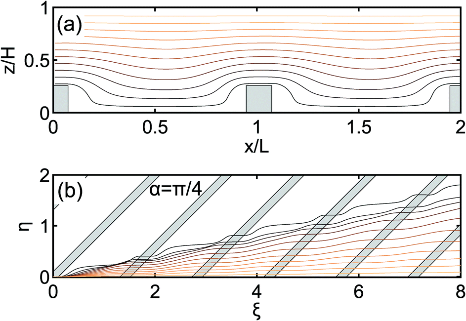

Fig. 2 xz (a) and ηξ (b) projections of electroosmotic flow field streamlines calculated for α = π/4. The colors of streamlines correspond to their height above the center of a ridge: from black at z = e to copper at z = H. Gray rectangles show the position of the ridges.

Near a grooved texture, the liquid deflects from the direction of the electric field E (Fig. 2(b)). To quantify this deflection, we introduce an angle β, which defines the ratio of the velocity components, averaged over a period, so that tan β = u_η/u_ξ for each streamline with a fixed starting point z above the center of the ridge. In Fig. 3(a), we plot the measured values of tan β as a function of the vertical coordinate z. We conclude that it decays nearly linearly, and vanishes completely at the upper flat wall. This suggests that a transverse shear flow has been generated in the channel. One can easily show that the ratio of transverse and forward flow rates is given by , and the value of Q_η/Q_ξ can be deduced from the simulation data. Our aim is to optimize the angle α between the directions of the grooves and the external electric field, so that Q_η/Q_ξ is maximal, providing the strongest transverse flow. The simulation results shown in Fig. 3(b) indicate that the optimal angle is α ≃ π/4, and this value of α has been used in all the subsequent simulations throughout the paper.

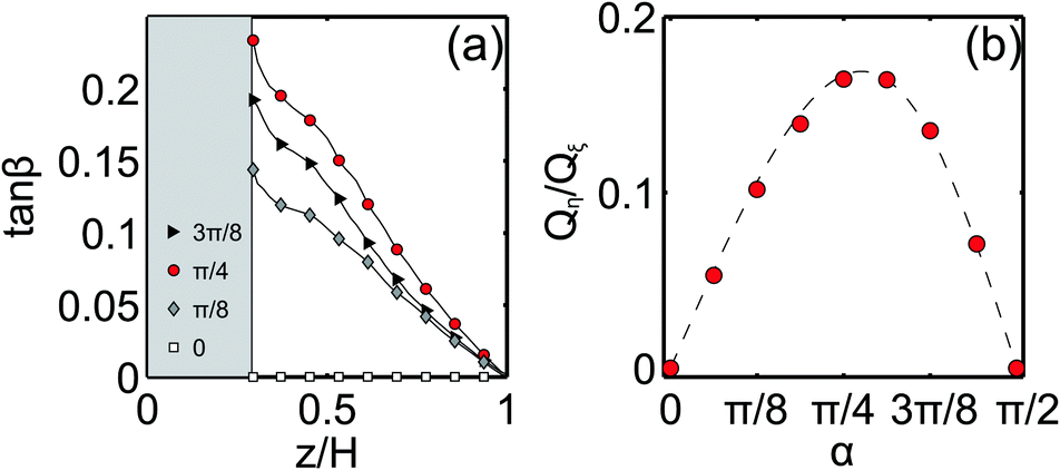Fig. 3 (a) tan β as a function of the streamline height above the center of a ridge calculated for α = 0, π/8, π/4, and 3π/4; (b) Q_η/Q_ζvs. α. Symbols show simulation data, and the dashed curve plots theoretical predictions, eqn (4).

We should also note that the value of Q_η/Q_ξ at a given α can be predicted theoretically. A precise discussion of the liquid flow rate in our microchannel (of a variable thickness) requires a complicated analysis. Here, we use an approach that is based on an approximate solution. To do so, we consider a plug forward flow with superimposed uniform transverse shear in a microchannel of a constant thickness. Such a simplification immediately leads to

where Q^⊥/Q^‖ denote the ratio of flow rates at α = π/2 and α = 0, and the prefactor A is included here to account for the influence of surface topology on the flow rate. We have fitted simulation data to eqn (4) taking A as a fitting parameter. The calculations are made using Q^⊥/Q^‖ = 0.72 obtained from simulations. The theoretical curve is included in Fig. 3(b), and the value of A = 1.04 has been obtained from fitting. A general conclusion from Fig. 3(b) is that the theoretical predictions are in good agreement with the simulation results confirming the validity of our simplified model. We also would like to stress that our theory provides a maximal value of Q_η/Q_ξ at α = 0.28π, which is in agreement with the simulation data.

4.2 Motion of single particles

We now turn to the simulation of single particles in the generated flow field. Immediately after the injection, different particles of the same size follow slightly different streamlines, which is due some difference in their lateral injection position. However, upon reaching the first ridge, all particles of the same size begin to follow the same streamline. This is the consequence of their finite size as illustrated in Fig. 4. Note that despite this focusing of different particles at the same streamline, we have observed some widening of the particle distribution at the end of the channel. Since the calculated displacement of the particles due to diffusion does not exceed 10⁻³a per period, the widening is likely caused by the initial lateral dispersion of particles.

Fig. 4 Sketch of the particle trajectories upon meeting the first groove wall.

In Fig. 5(a), we plot the yz-projections of the trajectories of the particle centers, which are periodical in the y-direction. One can see that the distance between the trajectories and the texture increase with the particle radius. We remark that particle trajectories (solid curves) slightly deviate from the streamlines (dotted curves), which is likely due to the finite size effects and non-uniformity of the flow near a grooved wall. Similar deviations in the lateral displacement of particles to the lateral displacement of streamlines have been found (Fig. 5(b)). We see a decay of lateral displacement of particles and streamlines with z, but tan β for particles is smaller. However, these differences are quite small, so we conclude that the fractionation of particles should be controlled by Q_η/Q_ξ.

Fig. 5 (a) Particle trajectories (solid curves) simulated for the particles of radii 5a, 4a, 3a, and 2a (from top to bottom) and streamlines of the electroosmotic flow field (dotted curves); (b) tan β for particles (circles) and streamlines (solid curve) as a function of their height above the center of a ridge.

In our computer experiment, we have also detected the rotation of particles near the edges of the grooved wall (Fig. 6). Namely, it has been found that particles located close to the corners of the grooves, where streamlines of the flow warp strongly, experience a significant torque. As a result, clockwise rotation near the upper corners (convex streamlines) and counter-clockwise rotation close to the lower corners (concave streamlines) of our rectangular grooves have been observed (Fig. 6(a)). Note that the absolute value of the angular velocity does not exceed 0.04τ⁻¹ (Fig. 6(b)). This implies that the rotation angles are π/2 and smaller. We can also conclude that smaller particles rotate faster since they move closer to the walls, where the curvature of streamlines is larger. The detected rotation does not strongly influence the translation of spherical particles. However, one can speculate that such a rotational motion could become important for the fractionation of non-spherical objects.

Fig. 6 (a) Illustration of rotation of particles near the corners of the grooves; (b) angular velocity of particles of radii 2a (solid black curve), 3a (solid red curve), 4a (solid grey curve), and 5a (dashed black curve).

4.3 Continuous sorting of the particles

Finally, we perform a full-scale computer experiment using a polydisperse suspension of particles. Fig. 7(a) shows the lateral random distribution of the particles in the inlet. The injected particles are translated forward by the flow. They focus at the first ridge, and then follow the distinct streamlines, defined by their size (see the Supplementary Video, ESI†). After 9 periods of grooves, their distribution becomes different as seen in Fig. 7(b). We conclude that the generated transverse flow has led to the fractionation of particles of different sizes. Note that in our computer experiment, we see some overlap between distributions of different size fractions at the outlet, but in a real experimental device, which would normally include dozens of texture periods, these fractions should be separated completely.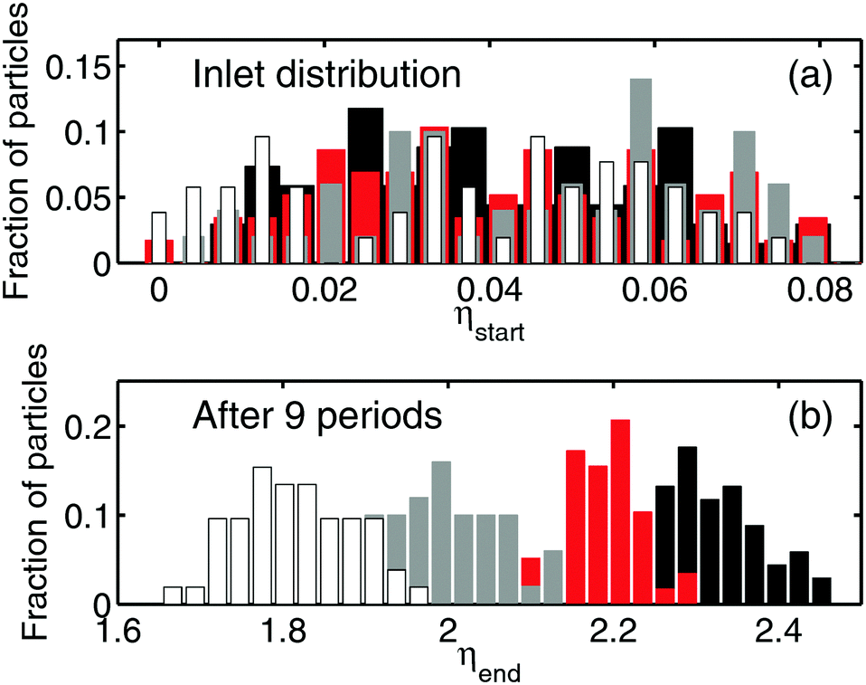

Fig. 7 Histograms of the lateral positions of particles η at the inlet (a) and after 9 periods of grooves (b). Black, red, gray, and white histogram bars correspond to the particles of radii R = 2a, 3a, 4a, and 5a.

Generally, the sensitivity of our system, i.e. the minimal size difference for particles to be separated, depends strongly on the length of the channel. Therefore, it is possible to separate particles of any, however small, size difference provided the channel is long enough. Note that surprisingly, the electric field amplitude does not affect the efficiency of separation. This is likely because it does not increase the shear rate of the secondary transverse flow. Therefore, by increasing the electric field we could only accelerate the separation, but not its selectivity.

5 Conclusions

We have suggested a novel concept of a continuous fractionation of particles in the electroosmotic flow. Our strategy is to generate a secondary transverse flow by using the grooved bottom wall of the microchannel. We have quantified this flow theoretically, and provided a detailed computer simulation study of the behavior of spherical particles near a grooved wall. Our computer experiment has also shown that different lateral displacements of particles of different sizes allow one to fractionate them efficiently. These results may guide the design of microfluidic devices for particle sorting.

Conflicts of interest

There are no conflicts to declare.

Acknowledgements

This research was partly supported by the Dynasty Foundation and by the Deutsche Forschungsgemeinschaft (DFG) through its Priority Programme 1726 “Microswimmers - from single particle motion to collective behavior”. We thank E. S. Asmolov, T. V. Nizkaya and S. R. Maduar for fruitful discussions at the initial stage of this study.

References

1. G. M. Whitesides, Nature, 2006, 442, 368.
2. T. M. Squires and S. R. Quake, Rev. Mod. Phys., 2005, 77, 977.
3. H. A. Stone, A. D. Stroock and A. Ajdari, Annu. Rev. Fluid Mech., 2004, 36, 381–411.
4. H. W. Hou, A. A. S. Bhagat, W. C. Lee, S. Huang, J. Han and C. T. Lim, Micromachines, 2011, 2, 319–343.
5. O. I. Vinogradova and A. V. Belyaev, J. Phys.: Condens. Matter, 2011, 23, 184104.
6. O. I. Vinogradova and A. L. Dubov, Mendeleev Commun., 2012, 22, 229–237.
7. J. G. Santiago, Anal. Chem., 2001, 73, 2353–2365.
8. S. Pennathur and J. G. Santiago, Anal. Chem., 2001, 77, 6772–6781.
9. R. B. Schoch, J. Han and P. Renaud, Rev. Mod. Phys., 2008, 80, 839.
10. A. Ajdari, Phys. Rev. E: Stat., Nonlinear, Soft Matter Phys., 2001, 65, 016301.
11. B. Rotenberg and I. Pagonabarraga, Mol. Phys., 2013, 111, 827–842.
12. N. Pamme, Lab Chip, 2007, 7, 1644–1659.
13. P. Sajeesh and A. K. Sen, Microfluid. Nanofluid., 2014, 17, 1–52.
14. P. S. Williams, T. Koch and J. C. Giddings, Chem. Eng. Commun., 1992, 111, 121–147.
15. J. McGrath, M. Jimenez and H. Bridle, Lab Chip, 2014, 14, 4139–4158.
16. D. Di Carlo, J. F. Edd, D. Irimia, R. G. Tompkins and M. Toner, Anal. Chem., 2008, 80, 2204–2211.
17. V. G. Levich, Physicochemical hydrodynamics, Prentice-Hall, 1962.
18. M. Z. Bazant and T. M. Squires, Phys. Rev. Lett., 2004, 92, 066101.
19. T. M. Squires and M. Z. Bazant, J. Fluid Mech., 2004, 509, 217–252.
20. J. Zhou, R. Schmitz, B. Dünweg and F. Schmid, J. Chem. Phys., 2013, 139, 024901.
21. D. Feldmann, S. R. Maduar, M. Santer, N. Lomadze, O. I. Vinogradova and S. Santer, Sci. Rep., 2016, 6, 36443.
22. J. I. Molho, A. E. Herr, B. P. Mosier, J. G. Santiago, T. W. Kenny, R. A. Brennen, G. B. Gordon and B. Mohammadi, Anal. Chem., 2001, 73, 1350–1360.
23. Z. Wu, A. Q. Liu and K. Hjort, J. Micromech. Microeng., 2007, 17, 1992.
24. A. V. Belyaev and O. I. Vinogradova, Phys. Rev. Lett., 2011, 107, 098301.
25. S. S. Bahga, O. I. Vinogradova and M. Z. Bazant, J. Fluid Mech., 2010, 644, 245–255.
26. T. M. Squires, Phys. Fluids, 2008, 20, 092105.
27. Q. Zhou and C.-O. Ng, Fluid Dyn. Res., 2014, 47, 015502.
28. M. Kim, A. Beskok and K. Kihm, Exp. Fluids, 2002, 33, 170–180.
29. J. Hahm, A. Balasubramanian and A. Beskok, Phys. Fluids, 2007, 19, 013601.
30. S. Kang and Y. K. Suh, Microfluid. Nanofluid., 2009, 6, 461–477.
31. D. Halpern and H.-H. Wei, Langmuir, 2007, 23, 9505–9512.
32. E. S. Asmolov, A. L. Dubov, T. V. Nizkaya, A. J. C. Kuehne and O. I. Vinogradova, Lab Chip, 2015, 15, 2835–2841.
33. V. Lobaskin, B. Dünweg and C. Holm, J. Phys.: Condens. Matter, 2004, 16, S4063.
34. T. Y. Molotilin, V. Lobaskin and O. I. Vinogradova, J. Chem. Phys., 2016, 145, 244704.
35. V. Lobaskin and B. Dünweg, New J. Phys., 2004, 6, 54.
36. L. P. Fischer, T. Peter, C. Holm and J. de Graaf, J. Chem. Phys., 2015, 143, 084107.
37. M. Smoluchowski, Pisma Mariana Smoluchowskiego, 1924, 1, 403–420.
38. E. B. Cummings, S. Griffiths, R. Nilson and P. Paul, Anal. Chem., 2000, 72, 2526–2532.
39. H.-J. Limbach, A. Arnold, B. A. Mann and C. Holm, Comput. Phys. Commun., 2006, 174, 704–727.
40. P. Ahlrichs and B. Dünweg, Int. J. Mod. Phys. C, 1998, 09, 1429–1438.
41. J. Zhou and F. Schmid, J. Phys.: Condens. Matter, 2012, 24, 464112.
42. J. de Graaf, T. Peter, L. P. Fischer and C. Holm, J. Chem. Phys., 2015, 143, 084108.
43. J. D. Weeks, D. Chandler and H. C. Andersen, J. Chem. Phys., 1971, 54, 5237–5247.
44. J. Ramirez and A. Conlisk, Biomed. Microdevices, 2006, 8, 325–330.

---

Footnote

† Electronic supplementary information (ESI) available: A video file representing full-scale simulations of a polydisperse suspension. See DOI: 10.1039/c7sm00986k

---