A model-based technique for the determination of interfacial fluxes in gas–liquid flows in capillaries†
Received
11th October 2015
, Accepted 17th December 2015
First published on 20th January 2016
Abstract
We present a novel technique to quantify interfacial mass transfer in gas–liquid flows in capillaries. A model was developed which allowed the relationship between absorption fluxes and bubble size changes to be established. Depending on the observed absorption rate, two limiting and simplifying cases for low and high absorption rates were suggested. For both cases, the flux was viewed as an input function which optimally tracked the observed bubble velocity, bubble volume, and unit cell volume change. For the case of low absorption rates, the mass transfer coefficient can be assumed to be constant and the model was fitted to experimental data by adjusting the value of this mass transfer coefficient. The bubble velocities were extracted from flow images using the cross-correlation between measured signal intensities for nearby pixels. Bubble and unit cell volumes were not determined by individual tracking, but a probability density function was estimated for each location in the capillary which contains the bubble and unit cell sizes of all bubbles passed. This allows the model to be fitted to an ensemble of bubbles making the procedure more robust. The developed model was validated for CO2 absorption in a buffer solution, and then applied to CO2 absorption using the ionic liquid 1-ethyl-3-methylimidazolium acetate ([Emim][Ac]), which exhibits high absorption rates and less known thermophysical properties. The developed technique is able to quantify interfacial fluxes for a wide range of gas and liquid flow rates.
1. Introduction
Conventional equipment, such as counter-current packed bed columns or tray columns, works well if mass transfer is fast or reactions are intrinsically slow. However, if mass transfer is limited due to e.g. the high viscosity of one of the contacting phases, conventional equipment fails. Conventional contactors and reactors suffer from poor control of the hydrodynamics, besides limited mass transfer, often resulting in non-uniformities such as hot spots or broad residence time distributions leading to safety issues or lower yields.1 These drawbacks can be overcome by using microstructured reactors, which take advantage of their large interfacial area per unit volume to reduce mass and heat transfer resistances.2–5 Faster transfer rates allow precise temperature control, which reduces the risk of thermal runaway, hot spot formation and unwanted side reactions.
Gas–liquid mass and heat transfer is closely related to the hydrodynamics of the two-phase system. However, for contactors or reactors on the micro- or milliscale, these hydrodynamics differ significantly from the hydrodynamics inside large equipment. To characterize gas–liquid two-phase flow and the associated interfacial mass transfer, the absorption of CO2 in an alkaline solution has served as a model reaction in many studies,6–10 which aim to quantify the overall mass transfer coefficient kLa. Operating the microfluidic devices under Taylor flow results in efficient gas–liquid contact, as the continuous replacement of the liquid at the bubble caps due to internal circulation significantly increases the mass transfer rates.11,12 Multiple correlations exist to predict mass transfer rates in Taylor flow, and the most commonly used are presented in Table 1. Some correlations require detailed information such as slug length, gas hold-up, etc., while other correlations are based on dimensionless numbers requiring only knowledge of the physical properties of the gas and liquid phases, and their superficial velocities. Furthermore, these different mass transfer correlations are derived for different channel geometries, fluid systems and operating conditions, rendering the comparison of their accuracy difficult. These limitations of the correlations complicate the a priori prediction of interfacial mass transfer in cases where the thermophysical fluid properties are not known or change rapidly due to the absorption process. For these cases, a robust experimental technique to quantify interfacial mass transfer is necessary. Mass transfer in capillaries is often quantified by offline techniques. However, cumbersome treatment of entrance and exit effects, long sampling times, and the limitation to only overall (averaged) information have shifted attention to online measurement techniques.9,16–20 Nevertheless, the ability to probe local mass transfer rates is not always exploited. In addition, the proposed methods often require detailed knowledge of the physical fluid properties,9,18–20 reaction mechanisms,9 or the analytic form of the volumetric mass transfer coefficient.17
Table 1 Commonly used gas–liquid mass transfer correlations for Taylor flow in microreactors
| Reference |
Correlation for kLa |
| Berčič & Pintar13 |
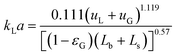
|
| van Baten & Krishna14 |
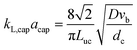
|
|
|
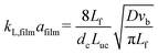 , Fo < 0.1 (short contact) , Fo < 0.1 (short contact) |
|
|
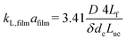 , Fo > 1 (long contact) , Fo > 1 (long contact) |
|
|
k
L
a = kL,capacap + kL,filmafilm |
| Vandu et al.15 |
|
| Yue et al.7 |
ShLadH = 0.084 Re0.213GRe0.937LSc0.5L |
| Kuhn & Jensen12 |
ShLadH = 20.8 + 0.07825 Re1.779GRe−0.1124LSc0.5L |
In the present study, we develop an image-based measurement technique together with a model to relate absorption fluxes and bubble size changes. Thereby, we are not tracking selected individual bubbles, but we are capturing an entire bubble ensemble (which can be non-uniform in its size distribution) in an extended section of a capillary. A probability density function is estimated for each location in the capillary which contains the bubble and unit cell sizes of all bubbles passed, and the bubble velocities are extracted from flow images using the cross-correlation between measured signal intensities for nearby pixels. The absorption model is validated for the well-studied system of CO2 absorption in a buffer solution, and then applied to CO2 absorption using the ionic liquid 1-ethyl-3-methylimidazolium acetate ([Emim][Ac]), which exhibits high absorption rates and less known thermophysical properties. The developed technique is able to quantify interfacial fluxes for a wide range of gas and liquid flow rates.
2. Methods
2.1. Experimental setup
The experimental setup is shown schematically in Fig. 1. Industrial grade CO2 (>99.5 vol%, Air Liquide) is introduced via a mass flow controller (Bronkhorst High-Tech EL-FLOW). Following the mass flow controller, a pressure gauge is used to estimate the pressure in the capillary, and a check valve (IDEX Health & Science, CV-3320) prevents liquid from entering the gas introduction system. The liquid (either the buffer solution or the ionic liquid) is introduced via a syringe pump (Chemyx Inc., Fusion 200). The two phases meet at the T-junction and the thus-established two-phase flow travels through a PTFE capillary with an inner diameter of 0.6 mm and a length of 0.27 m (buffer solution) or 0.3 m (ionic liquid).
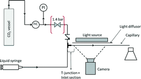 |
| | Fig. 1 Schematic of the experimental setup. | |
To prepare the buffer solution, a 1![[thin space (1/6-em)]](https://www.rsc.org/images/entities/char_2009.gif) :1 volume ratio of 0.1 M NaHCO3 and 0.1 M Na2CO3 in distilled water was used. The pH of the buffer was confirmed to be 9.9 using a pH meter (VWR 1000 L pHenomenal). 1-Ethyl-3-methylimidazolium acetate, [Emim][Ac], (≥97%, ≤0.5% water) was purchased from Sigma-Aldrich and used as-received. The physical constants used for the calculations are given in Table 2. Since the viscosity of [Emim][Ac] reported in the literature varies largely,21 a Peltier controlled double wall Couette geometry on an ARG2 rheometer (TA Instruments) was used for measuring the viscosity of our sample.
:1 volume ratio of 0.1 M NaHCO3 and 0.1 M Na2CO3 in distilled water was used. The pH of the buffer was confirmed to be 9.9 using a pH meter (VWR 1000 L pHenomenal). 1-Ethyl-3-methylimidazolium acetate, [Emim][Ac], (≥97%, ≤0.5% water) was purchased from Sigma-Aldrich and used as-received. The physical constants used for the calculations are given in Table 2. Since the viscosity of [Emim][Ac] reported in the literature varies largely,21 a Peltier controlled double wall Couette geometry on an ARG2 rheometer (TA Instruments) was used for measuring the viscosity of our sample.
Table 2 Physical constants (1 atm, 293 K) used for calculations
| Property/unit |
CO2 (ref. 22) |
Buffer solution22 |
[Emim][Ac] |
|
Own experiments; reported error is based on min/max values.
|
|
ρ/kg m−3 |
1.83 |
998 |
1098 (ref. 21) |
|
η/mPa s |
0.015 |
1.00 |
137 ± 3a |
|
σ/mJ m−2 |
|
72.7 |
42.9 (ref. 21) |
|
H/Pa m3 mol−1 |
|
2980 (ref. 22) |
— |
The imaging system consisted of a Photron FastCam Mini UX100 equipped with a Navitar NMV-25M1 lens. This broad angle lens was able to capture 40% of the capillary length, and the spatial resolution of the camera was cropped to the aspect ratio of the capillary, which resulted in images of 1280 × 24 pixel2. The frame rate was adjusted in the range of 2000–6250 Hz to obtain a similar pixel shift of the bubbles across all experiments, with a constant exposure time of 0.16 ms for all frequencies. A series of LEDs (Edmund Optics LED 6′′ High Intensity Line, White) was used as background lighting, together with a paper-based light diffusor to homogenize the light.
2.2. Data extraction
Bubble lengths, unit cell lengths and bubble velocities are measured using the recorded images of the capillary. This section discusses (i) the image pretreatment needed for successful data extraction, (ii) how the bubble velocities are extracted in a fast and efficient way, and (iii) how the bubble and unit cell lengths, or equivalently, the bubble and unit cell volumes are determined.
Step 1: the images are transformed to arrays of greyscale values (where 0 corresponds to black and 255 corresponds to white). The greyscale values are then summed along the cross-section of the capillary. This makes data handling easier and reduces the amount of data that have to be stored. The vectors obtained for each frame are concatenated in a matrix. This matrix allows data to be accessed in both time- and space-sliced forms by looking at the individual rows or columns (see Fig. 2a). Time-sliced data represent the data provided by a single frame; space-sliced data, on the other hand, represent the observation of greyscale values for different times at a certain, fixed position.
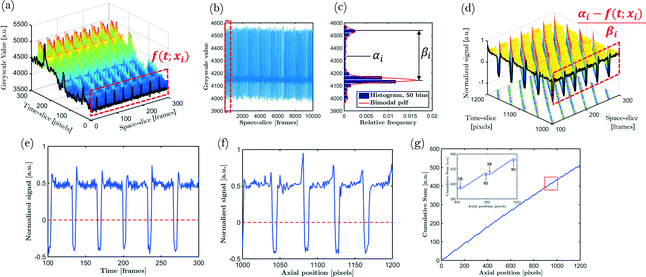 |
| | Fig. 2 Pretreatment of the raw data. (a) Time- and space-sliced view of the raw data, (b) space-sliced view for all recorded frames at a particular position xi, (c) the corresponding relative frequency plot, (d) raw data after centering and normalization, (e) and (f) a close-up of the individual time-sliced and space-sliced data, and (g) the cumulative signal of time-sliced data indicating bubble–slug (BS) and slug–bubble (SB) transitions. | |
Step 2: variations in background illumination result in a variable baseline. Further processing is simplified by (i) removing this baseline and (ii) removing intensity differences between slugs and bubbles with respect to this baseline. Note that while time-sliced data suffer from inhomogeneous lighting, space-sliced data are free of this problem (see Fig. 2a). Hence, data centering and normalization using space-sliced data is easier. Centering the data requires the 0-line to be specified. From a practical point of view, it is easy if this 0-line corresponds to the transition between bubbles and slugs. By inspecting Fig. 2b, which shows space-sliced data, it can be seen that the majority of the data points lie in two narrow greyscale regions depicting the slugs and bubbles and only a small fraction of the data points are situated in intermediate regions.
This is illustrated by the corresponding bimodal histogram (Fig. 2c) of the greyscale values. The center between the peaks of the bimodal distribution is set to zero. By dividing the signal by the distance between both peaks, the signal is normalized. The final normalized time- and space-sliced results are shown in Fig. 2d–f.
Step 3: a calibration curve is constructed for each experiment. By placing a ruler with regularly spaced marks with known distance, small misalignment errors and lens distortions can be corrected. The distance in pixels between two calibration marks is determined by the distance between two greyscale peaks. The process is illustrated in Fig. 3.
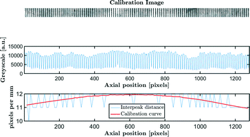 |
| | Fig. 3 Construction of the calibration curve. | |
Step 4: bubble velocities are determined using the cross-correlation between two time- or space-sliced datasets, depending on whether the velocity changes as a function of time or space are computed. In the following, we consider time-sliced data f(x) with the autocorrelation function:
| | | (f ★ f)(ξ) = ∫∞−∞f(x)f(x + ξ)dx | (1) |
Since Taylor flow results in a periodic function f(x) with period X, the autocorrelation will be maximum at ξ = 0 but also at ξ = ±X, ±2X, etc. After a certain time interval, Δt, the original signal f(x) has moved a distance Δx and a new signal g(x) is measured. Cross-correlating g(x) and f(x) results in:
| (f ★ g)(ξ) = ∫∞−∞f(x)g(x + ξ)dx = ∫∞−∞f(x)f(x − Δx + ξ)dx = (f ★ f)(ξ − Δx) |
Hence, (f ★ g) (ξ) reaches its maximum value at ξ = Δx + nX for integer n. This shows that the cross-correlation function between the original signal f(x) and the signal g(x) (Δt frames later) can be used to determine Δx. The bubble velocity can then be calculated as:
| |  | (2) |
To obtain an accurate value for Δx, a Δt value corresponding to 2 to 20 frames is needed. However, a typical measurement set consists of 4000 to up to 20000 image frames per experiment, and consequently Δx can be estimated multiple times during the entire experiment. Consequently, if a dynamic experiment is performed, different values for Δx are obtained, i.e. the use of time-sliced data allows resolution of temporal variations in the bubble velocity. When space-sliced data are used, a similar result is obtained: if f(t) is the signal measured at a position x in the capillary and g(t) is the signal measured Δx from x, then the cross-correlation between f(t) and g(t) can be used to measure the shift Δt between both signals. The resulting bubble velocity is then:
| |  | (3) |
To obtain an accurate value for Δt, a Δx value corresponding to 5 to 30 pixels is needed. As the width of a frame is 1280 pixels, this approach can measure spatial variations in the bubble velocity. As is shown, to calculate the bubble velocity, either a time-sliced or space-sliced approach can be used. If variations in bubble velocities with time are expected, then the time-sliced approach should be used. However, in the following, we only consider steady-state experiments and avoid temporal variations in bubble velocities. Therefore, the space-sliced approach is used. The spatial distance Δx between both signals is varied for each position x in the capillary. This is mainly to check if different spatial distances indeed give the same bubble velocity, i.e. vb(x) is independent of Δx. Due to discretization errors, the bubble velocities for Δx for each position x vary slightly. The discretization errors occur since pixels and frames always have an integer value. For example, suppose the true velocity is 1.8 pixels per frame. If Δx is chosen to be 5 pixels, then, using the cross-correlation, Δt will be 3 frames. Hence, the measured velocity will be 1.67 pixels per frame. If Δx is chosen to be 6 pixels, then, using the cross-correlation, Δx will also be 3 frames, and the measured velocity will be 2 pixels per frame. To reduce this error, an average of multiple vb(x, Δx) for different values of Δx is used to obtain the true value of vb. For the given example, it can be seen that the average between 2 pixels per frame and 1.67 pixels per frame is 1.84 pixels per frame, which is already close to the real velocity, 1.8 pixels per frame. However, due to the strong correlation of the discretization error between bubble velocities for different Δx values, the average bubble velocity still suffers from inaccuracies. The additional smoothing required is realized by using a Savitzky–Golay filter.23
Step 5: the bubble and unit cell volumes are calculated conveniently by taking the cumulative sum of a time-sliced, centered and normalized signal. Since centering corresponds to placing the 0-line at the phase interface, the cumulative sum increases where the signal indicates a bubble and decreases where the signal indicates a liquid slug. Local maxima in this cumulative sum correspond to bubble–slug (BS) transitions and local minima correspond to slug–bubble (SB) transitions (see Fig. 2g). Since the locations of the maxima and minima never exactly correspond to the intersection of the 0-line in Fig. 2f due to the discrete nature of the signal, linear interpolation is used to estimate this intersection. The distances between maxima and minima are used to determine the bubble lengths and unit cell lengths. The bubble volume and unit cell volume can be calculated if an ideal bubble shape of two hemispherical caps connected by a cylinder is assumed. Each bubble and unit cell length is stored together with the position of the bubble center and unit cell center for each frame, respectively.
Step 6: the capillary is divided into a certain amount of bins. Using the positions for each bubble and unit cell, the corresponding volumes are assigned to a bin. Hence, for each position in the capillary, a distribution of the bubble and unit cell volumes that have passed this bin during the experiment is determined. This distribution can be used to track the change in volume of an ensemble of bubbles with a given initial volume. This is visualized in Fig. 4 where bubbles travel from left to right. If α is a cumulant of the measured distribution at the left hand side (x1) of the frame, this denotes the boundary between all bubbles smaller and larger or equal to the bubble size Vbα(x1). The bubble volume at x > x1 can, in principle, be predicted using the set of ordinary differential eqn (4)–(8) given the initial state of the bubble at x1. It is also known that solutions of these initial value problems are unique. A consequence is that the solutions of initial value problems will never intersect for x < ∞. Hence, a bubble with an initial volume of Vbα(x1) ± δVb will always remain smaller (−), or larger (+), than the reference bubble with volume Vbα even after it has reached position x > x1. This means that the bubble volume, Vbα(x), remains the α-cumulant of the distribution at position x. Hence, the evolution of the α-cumulant is equal to the evolution of a bubble with initial volume Vbα(x1). The use of cumulants (such as, for example, the median value or the percentiles) of the measured bubble distributions has two advantages compared to using the average of the measured distributions, both illustrated in Fig. 4. Firstly, the average bubble volume does not necessarily correspond to an actual bubble which has traveled through the capillary. In this case, the average bubble volume may not be representative of the majority of the bubbles if few outliers are present. Secondly, the average value does not necessarily correspond to the actual evolution of the bubble volume. Hence, median bubble volumes and unit cell volumes are reported instead of average values.
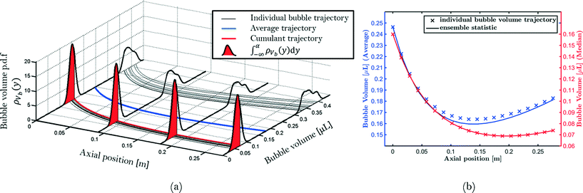 |
| | Fig. 4 Simulated bubble volume trajectories using eqn (4)–(8) with  showing (a) the relationship between individual bubble trajectories, evolution of the estimated probability density function (p.d.f.) and ensemble statistics such as cumulants and averages, and (b) the comparison between ensemble statistics and actual bubble volume trajectories. showing (a) the relationship between individual bubble trajectories, evolution of the estimated probability density function (p.d.f.) and ensemble statistics such as cumulants and averages, and (b) the comparison between ensemble statistics and actual bubble volume trajectories. | |
2.3. Model-based fitting
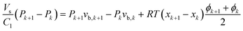
The general model equations for the profiles of all relevant quantities for segmented flow are given by:| |  | (4) |
| | 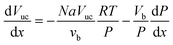 | (5) |
| |  | (6) |
| |  | (7) |
| |  | (8) |
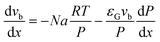
where the absorption flux N is given by:where kL is the liquid side mass transfer coefficient, E is the chemical enhancement factor and ceq is the equilibrium absorbent concentration. For a sparingly soluble gas, it is assumed that Henry's law (ceq = P/H) is valid.
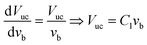
The total pressure drop, taking into account the effect of deceleration, is given by eqn (8). However, even for very fast absorption rates, the volumetric absorption flux Na is smaller than 103 mol m−3 s−1. Hence, the contribution of the deceleration term  (O(103)–O(104) Pa m−1) is small compared to the total pressure drop (O(105)–O(106) Pa m−1) for small capillaries. In addition, εGρLvb2/P (O(10−3)) is much smaller than 1. As a result, only τS/A is retained. This contribution is implicitly assumed to be a combination of both the viscous and the Laplace pressure drop. If eqn (5) is divided by eqn (6), the resulting differential equation simplifies to:
| |  | (10) |
Therefore, the general model equations suggest that there is a linear relationship between the unit cell volume of a bubble and its corresponding velocity. The constant C1 can be estimated from regressing Vuc with vb. Since Vuc = Vb + Vs, Vs can be found by regressing Vb with vb:
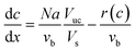
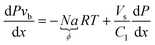
Generally, it is possible that kLaE and τ are not constant throughout the capillary. In addition, it is possible that information concerning solubility and chemical reactions is lacking. However, the absorption flux N or the volumetric absorption flux Na = ϕ can still be determined. In this case, ϕ is a function of the position of the bubble in the capillary. If eqn (6) is multiplied by P and the linear relationship between Vuc and vb is used, then we obtain:
| |  | (12) |
In principle, if P and vb are known as functions of x, the volumetric absorption flux ϕ can be found by substituting the experimental measurements into eqn (12). However, numerical differentiation of experimental data amplifies the noise to a level which precludes quantitative analysis.
We propose to find ϕ by introducing the optimality condition (O.C.):
| |  | (13) |
and finding the function
ϕ which minimizes this optimality condition. The following expression for
L is used:
| | 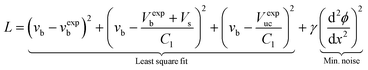 | (14) |
L was chosen to consist of two parts. The squared differences between predicted and measured quantities correspond to the optimality criterion used in least-squares fitting procedures. However, since the volumetric flux
ϕ has to be determined for every position
x, only using the least-square term will result in fitting the model almost exactly to the data (and its noise). Hence, only using the least-square fit term in
eqn (14) will give problems similar to direct numerical differentiation. The reason is that when the least-squares fitting procedure changes the volumetric flux
ϕ(
x) in order to fit the model with experiments, there is no bound on the value of the flux at
ϕ(
x + Δ
x). In order to avoid the flux having very large oscillations, the rate of change of
ϕ(
x) must be limited.
In the following, let ϕ(x) be the fitted volumetric flux determined in position x. For the next data point (at x + Δx), the fitted volumetric flux is found to be ϕ(x + Δx). Generally, ϕ(x) is not equal to ϕ(x + Δx). However, this could be due to either experimental noise or a genuine change in the flux. Hence, we do not impose a limit on ϕ(x + Δx) − ϕ(x). At x + 2Δx, a volumetric flux ϕ(x + 2Δx) is fitted. If the flux increases or decreases, we expect the acceleration/deceleration of the flux to be relatively slow. This means that for sufficiently small Δx,
| | 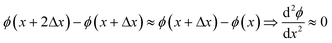 | (15) |
In this study, Δx was as small as a half bubble length. This means that after moving 2Δx, the bubble has traveled its own length. It is unlikely that within this distance, the rate of flux increase/decrease changes drastically. In contrast to the above, large values for ϕ′′(x) indicate that ϕ is being fitted to noise. Hence, by adding this term to L, the degree of fitting to noise is incorporated. In eqn (14), this term is squared in order to make L positive definite.
The relative contribution of both fitting and noise minimization effects can be tuned by adjusting the value of γ. If γ is very small, the error between predicted and measured data becomes important. Too small values of γ will fit ϕ to noise. In contrast, if γ is large, reducing fluctuations in the slope of ϕ becomes important. If γ is too large, the model becomes insensitive to the measurements and the fitted result will not follow the trends in the measured data. In our procedure, the fitted flux at xi is linearly extrapolated to predict the experimental data for a window of the next n data points xi+1, xi+2, …, xi+n. After calculating the sum of squared errors between predicted and experimental data, the process is repeated for the flux extrapolated at xi+1. The value for γ is then determined by the value giving the lowest total sum of squared errors for all i (see ESI† 2.2 for further details).
In summary, if L is given by eqn (14), the fitting procedure tries to (i) minimize the difference between the predicted and measured velocity, bubble volume and unit cell volume, and (ii) avoids fitting to noise by penalizing frequent changes in the slope of ϕ.
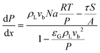
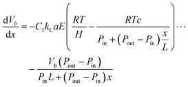
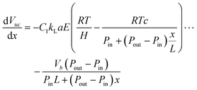
It should also be noted that a model is required to predict the pressure at every point in the capillary. Since the absorption rate can be high enough to alter the hydrodynamics, it is not necessarily true that the pressure gradient remains constant. However, if a pressure drop model is proposed and if it is assumed that ϕ is linear between the measurement points xk, eqn (12) can be integrated. After some rearrangement, this results in a recursive set of algebraic equations:
| |  | (16) |
The optimal flux can be determined very efficiently numerically by rewriting the discretized model (eqn (16)) and optimality criterion (eqn (13)) in standard quadratic form:
where
x represent the unknowns,
H and
A are constant matrices and
b is a constant vector.
For the case of low absorption rates, the bubble size changes are sufficient to be observed, but not sufficient to influence the hydrodynamics. Hence, it can be assumed that the pressure drop per unit length and the liquid side mass transfer coefficient remain constant. In addition, it is reasonable to assume that the interfacial area per unit reactor volume a remains constant as well. The enhanced volumetric mass transfer coefficient kLaE and slug volumes Vs are found by non-linear least-squares regression with experimental measurements of Vb, Vuc and ΔP.
Minimize:
| | 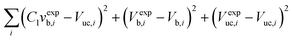 | (19) |
Subject to:
| |  | (20) |
| |  | (21) |
| | 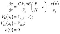 | (22) |
However, if c is not measured directly, H and the kinetic parameters in r(c) cannot be determined uniquely from a fitting procedure and must be supplied a priori. Note that Vs can be determined from either the non-linear least-squares regression itself (eqn (19)) or the average difference between Vexpuc and Vexpb. Although determining Vs with eqn (19) is less precise, it provides a check if the solution of the fitting procedure agrees at least partially with the experiment. In addition, since the first data points contain noise, Vuc,1 is also treated as an unknown parameter.
Frequently, kLa is determined using
| | 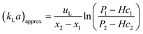 | (23) |
However, this equation is not the exact solution of eqn (22). In order to assess the difference between the fitting procedure (eqn (19)) and eqn (23), c can be calculated from the results of the fitting procedure and subsequently substituted in eqn (23). In addition, if it is assumed that no reactions proceed at any appreciable rate, the fitted flux that minimizes eqn (13) can be used to calculate c and find kLa through eqn (23). This allows a comparison of the proposed procedures with each other and the literature.
3. Results
3.1. Data extraction
Fig. 5 compares the averaged bubble velocity, the smoothed bubble velocity and the manually determined bubble velocity. The smoothing filter (Savitzky–Golay filter) uses a first-order polynomial with a window of 151 smoothing points. The smoothed bubble velocity is compared with the manual determination of the bubble velocity, i.e. counting the number of pixels the bubble has traveled within a certain amount of frames. Excellent agreement between both values is observed.
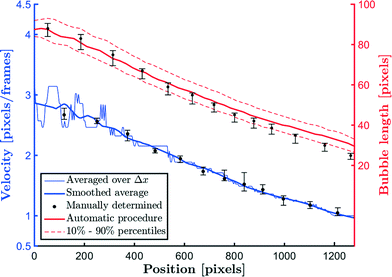 |
| | Fig. 5 The bubble velocities averaged over different values of Δx, the smoothed velocity, and the automatically determined bubble length compared with manually tracked bubbles for [Emim][Ac] (![[q with combining dot above]](https://www.rsc.org/images/entities/i_char_0071_0307.gif) G = 7 mln min−1, G = 0.3 ml min−1). G = 7 mln min−1, G = 0.3 ml min−1). | |
Fig. 5 also compares the bubble lengths determined using the automatic procedure with the bubble lengths of 10 manually tracked bubbles. The error bars denote the 10% and 90% percentiles. The comparison is reasonable, except for small bubble lengths. However, for that case, the thickness of the interfacial area relative to the bubble length is an important factor. In both the automatic and manual cases, the interface location needs to be determined, and since the manual case relies on human judgment, it is less accurate.
It is also worth noting that eqn (4)–(6) predicted linear relationships between the bubble volume, unit cell volume and bubble velocity. These linear relationships are confirmed with our experimental data (see ESI† 2.1 for details).
3.2. CO2 absorption in a Na2CO3/NaHCO3 buffer
Fig. 6a shows a sample picture taken from the capillary for CO2 absorption in the carbonate buffer for G = 4 mln min−1 and L = 4 ml min−1. The low absorption rate procedure can be used in order to determine the volumetric mass transfer coefficient kLaE if it is assumed that r(c) ≈ 0 mol m−3 s−1, H = 2980 m3 Pa mol−1,22 and E ≈ 1.7 Comparing the measured volumetric mass transfer coefficient with literature correlations (see Fig. 7) results in a good agreement with the correlation of Berčič & Pintar13 (Fig. 7(a)). Since the liquid film surrounding the Taylor bubbles was nearly saturated in their experiments, this suggests that the liquid film does not contribute much to kLa. Similarly, if only the bubble cap contribution of van Baten & Krishna14 is retained, the agreement with experiments is far better (Fig. 7(c)). In contrast, the correlation of Vandu et al.15 overpredicts the measured kLa since it essentially is the correlation of van Baten and Krishna without the bubble cap contribution (Fig. 7(d)). The remaining correlations are purely empirical correlations based on dimensionless quantities and cannot provide as much information on the absorption process. Since the applied flow rates and observed flow patterns correspond better with the experimental conditions used by Kuhn & Jensen,12 the agreement between the correlation and experiment is better compared to the correlation proposed by Yue et al.7 Next to the fact that these correlations cannot take the specific flow patterns (bubble length, velocity, etc.) into account, the discrepancy between measured and predicted kLa can mostly be attributed to the difference in experimental setups, which includes the use of Y-junctions instead of T-junctions,7 using rectangular channels,7 or using a meandering/serpentine channel.12
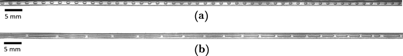 |
| | Fig. 6 Sample pictures of the capillary section for CO2 absorption in (a) the buffer solution and (b) [Emim][Ac]. | |
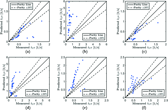 |
| | Fig. 7 Predicted vs. measured kLa for the correlation of (a) Berčič & Pintar,13 (b) van Baten & Krishna,14 (c) van Baten & Krishna, without film contribution, (d) Vandu et al.,15 (e) Yue et al.7 and (f) Kuhn & Jensen.12 | |
Fig. 8 compares the kLa values obtained from the least-squares fitting procedure (eqn (19)) with (kLa)approx obtained from eqn (23) after finding c from either kLa or the flux fitting procedure (eqn (13)). Using eqn (23) generally results in smaller kLa values compared to the least-squares fitting procedure (eqn (19)) even if the c-profiles are predicted by eqn (22). This is a consequence of the incorrect incorporation of the decreasing pressure drop in eqn (23). Except for some outliers at higher mass transfer rates, similar values for kLa are obtained from c-profiles predicted directly from the fitted flux or from eqn (22). At higher mass transfer rates and smaller slug volumes, however, the liquid slugs approach saturation and small differences in the predicted concentration c2 in eqn (23) will result in large kLa differences.
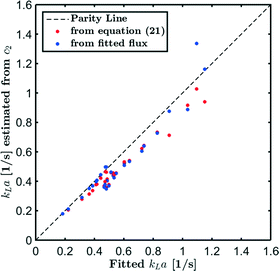 |
| | Fig. 8 Comparison between kLa values obtained by different methods. | |
3.3. CO2 absorption in 1-ethyl-3-methylimidazolium acetate
Fig. 6b depicts an example of CO2 absorption in [Emim][Ac] for G = 7 mln min−1 and L = 0.3 ml min−1. A rapid decrease in the bubble volume is observed, which is quantified in Fig. 9. This figure shows that if the gas flow rate is kept constant, the volume of the bubbles entering the camera frame decreases dramatically. The data also indicate that in the initial section (<15% of the capillary length), a large part of the absorption process has already taken place as we observe a spread in the initial bubble volumes (which should be similar for the same gas flow rate). As expected, an increase in the gas velocity increases the bubble volumes entering the camera frame. Fig. 9 also shows nearly parallel bubble volume profiles for small bubble volumes and for bubbles further downstream in the capillary. In contrast to this, steeper profiles are observed at the beginning of the capillary section as the liquid flow rates decrease. This could indicate a change in the absorption mechanisms. If the bubble volume approaches πdc3/6 (indicated by the red line in Fig. 9), the described procedure for determining the bubble volume yields unreliable results as it relies on the specific elongated shape of the gas bubbles, and hence the data processing is stopped upon reaching this condition. To determine the absorption flux, the pressure drop has to be known. In the case of slow CO2 absorption, the bubbles did not change in size rapidly and it could safely be assumed that the pressure drop remains constant along the channel length. However, for fast absorption in [Emim][Ac], this is not necessarily true. Consequently, a pressure drop model has to be used in order to use eqn (16), and in principle, any model can be incorporated. In this study, the pressure drop model proposed by Kreutzer et al.24,25 is used to determine the axial pressure gradient:| | 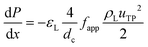 | (24) |
| | 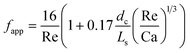 | (25) |
However, using eqn (10), it appears that even in this case the pressure drop is constant:
| | 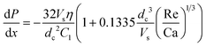 | (26) |
with Re/Ca only depending on constant quantities. Since this pressure drop model was specifically developed for Taylor flow, it cannot be applied if the bubble volume is smaller than π
dc3/6. For this case, it is assumed that the single-phase pressure drop as predicted by the Hagen–Poiseuille equation holds
| |  | (27) |
If
xT denotes the position at which
Vb = π
dc3/6, then the total pressure drop across the capillary can be estimated from a weighted average of
eqn (26) and
(27). The measured pressure drop and predicted pressure drop along the entire capillary are shown in
Fig. 10.
 |
| | Fig. 9 Evolution of the bubble volume for CO2 absorption in [Emim][Ac]. | |
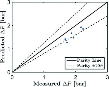 |
| | Fig. 10 Comparison between predicted and measured pressure drop for CO2 absorption in [Emim][Ac]. | |
The agreement is very reasonable when the approximations in the equations and the uncertainties in the physical constants of [Emim][Ac] are taken into account. It also follows that the pressure drop model can be reliably used to estimate the pressure for determining the volumetric flux.
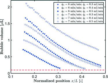
The measured flux in the CO2–[Emim][Ac] experiments for different gas and liquid flow rates is shown in Fig. 11. For higher liquid flow rates, higher volumetric fluxes are observed. The highest volumetric flux is found for the bubbles entering the camera frame. As the absorption process continues and the bubble volume decreases, the volumetric flux also decreases. However, for lower liquid flow rates, we observe a changing trend in the volumetric flux as the bubbles decrease in size indicating that the absorption mechanism changes for these bubbles. This corresponds to the findings from Fig. 9. In comparison, Fig. 12 depicts the evolution of the absorption flux as a function of the normalized gas void fraction, which is defined as the local gas void fraction divided by the theoretical gas void fraction at the T-junction. This also shows that in the short inlet section (not captured by the camera frame), a significant amount of CO2 has already been absorbed. As a result, the bubble volume and velocity have been substantially reduced at the location where the measurement is started.
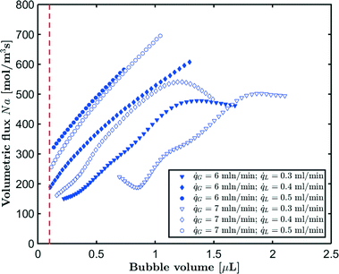 |
| | Fig. 11 Local absorption flux as a function of bubble volume for CO2 absorption in [Emim][Ac]. | |
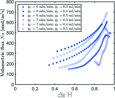 |
| | Fig. 12 Local absorption flux as a function of normalized gas void fraction for CO2 absorption in [Emim][Ac]. | |
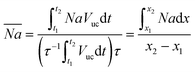
Although it is possible to measure the local flux, often only an average value is desired as it is easier to interpret and use. The average volumetric flux can be calculated as the total amount of CO2 that is absorbed in a unit cell whilst a single bubble travels through the captured capillary section. Since the unit cell itself changes, an average value for the unit cell volume is calculated according to:
| |  | (28) |
with
τ as the residence time of the bubble in the capillary section and making use of the linearity between the unit cell volume and the bubble velocity (
eqn (10)). This definition reduces to the average of the measured volumetric flux in a stationary reference frame. The residence time is measured within the camera frame or for bubbles larger than π
dc3/6. For slow absorption, the absorption rate is often compared to the residence time, as shorter residence times (
i.e. higher bubble velocities) typically increase absorption rates. In this case, the residence time is viewed as independent of the absorption flux. However, in the case of very high absorption rates, the residence time itself is influenced by the absorption rate and is not a suitable parameter to compare different experiments.
Fig. 13 instead uses Δ
x/
uL as a characteristic timescale since it is not influenced by the absorption rate and remains constant in the camera frame. In this expression, Δ
x denotes the distance the Taylor bubble (
Vb > π
dc3/6) traveled in the camera frame. From
Fig. 13, it can be clearly seen that as Δ
x/
uL increases, the average flux decreases (see ESI
† 3). However, due to the fast absorption process, the hydrodynamic conditions change rapidly in the capillary, which complicates the determination of the effect of other parameters. Furthermore, and as discussed above, the contacting zone and the short inlet section could not be captured with the camera, which results in a lack of information about the interfacial flux in this section. The influence of this effect can be seen in the volumetric flux, which for the inlet conditions of
G = 6 mln min
−1 and
L = 0.3 ml min
−1 is found to be lower than the corresponding volumetric flux for
G = 7 mln min
−1. From
Fig. 11 and
12, it can be seen that for
G = 6 mln min
−1 the bubbles have already largely been absorbed compared to
G = 7 mln min
−1. This is further quantified by the value of the gas void fraction upon entering the camera frame, which is already significantly lower compared to the initial gas void fraction (
εG/
εG(0) = 0.87). Hence, further development of the proposed techniques would require that the contacting region and the inlet section are captured by the camera.
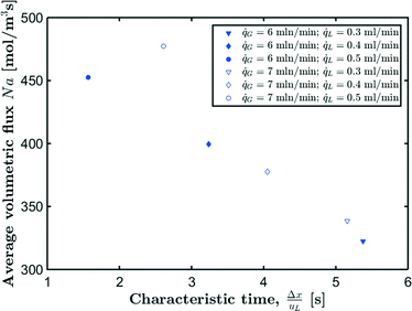 |
| | Fig. 13 Average absorption flux as a function of Δx/uL for CO2 absorption in [Emim][Ac]. Reported flow rates are the set values at the inlet. | |
4. Conclusions
A model-based technique has been developed to quantify interfacial mass transfer in gas–liquid flows in capillaries. The underlying model relates absorption fluxes to bubble size changes, which then allows either the mass transfer coefficient kLa (if all thermophysical properties of the fluids are known) or the volumetric flux Na to be computed.
The most notable feature of the technique presented in this paper is that an entire ensemble of bubbles is captured over a long capillary section. This allows the absorption process to be monitored based on a probability density function rather than a discrete description of individual bubbles. Consequently, fast absorption processes in which the hydrodynamics of the two-phase flow change can be readily quantified rapidly. Furthermore, the developed technique determines the interfacial flux in an integral way, which also increases its precision.
In terms of the hydrodynamics of the gas–liquid flow, it is observed that the model equations predict a linear correlation between the bubble volume, unit cell volume and bubble velocity for both slow and fast absorption processes. This predicted linearity was confirmed with our experimental data.
The developed model was validated for CO2 absorption in a Na2CO3/NaHCO3 buffer solution (slow absorption with known thermophysical fluid properties), and the observed mass transfer coefficient kLa agrees well with correlations from the literature. We then quantified the interfacial flux of CO2 absorption in the ionic liquid 1-ethyl-3-methylimidazolium acetate ([Emim][Ac]), which exhibits high absorption rates and less known thermophysical properties. It was shown that the developed technique is able to quantify interfacial fluxes for a wide range of gas and liquid flow rates.
The observations also highlight the importance of capturing the contacting zone for fast absorption processes, as the interfacial flux in this rather short section of the capillary is not negligible.
Nomenclature
Roman symbols
|
a
|
Gas–liquid interfacial area per unit volume
|
|
A
|
Cross-sectional area
|
|
c
|
Concentration in molar units
|
|
d
|
Diameter
|
|
D
|
Molecular diffusivity
|
|
E
|
Chemical enhancement factor
|
|
f
app
|
Apparent Fanning friction factor
|
|
f(x), g(x) |
Generic functions
|
|
H
|
Henry coefficient in [Pa m3 mol−1]
|
|
k
|
Mass transfer coefficient
|
|
L
|
Length
|
|
N
|
Flux
|
|
P
|
Pressure
|
| ΔP |
Pressure drop
|
|
|
Volumetric flow rate
|
|
r
|
Reaction rate
|
|
R
|
Ideal gas constant
|
|
S
|
Cross-sectional perimeter
|
|
t
|
Time
|
|
T
|
Absolute temperature
|
|
u
|
Superficial velocity
|
|
v
|
Velocity
|
|
x
|
Axial position in capillary
|
|
x
1
|
Position where bubbles enter the camera frame
|
|
x
T
|
Position where Taylor flow stops
|
|
x
2
|
Position where bubbles leave the camera frame
|
Greek symbols
|
γ
|
Fitting constant
|
| Δ |
Difference
|
|
δ
f
|
Liquid film thickness
|
|
ε
|
Volumetric fraction
|
![[small epsi, Greek, dot above]](https://www.rsc.org/images/entities/i_char_e0a1.gif)
|
Transport fraction
|
|
η
|
Viscosity
|
|
ρ
|
Density
|
|
σ
|
Surface tension
|
|
τ
|
Shear stress; residence time, defined as (x2 − x1)/uTP
|
Subscripts and superscripts
| b |
Bubble
|
| c |
Capillary
|
| f |
Liquid film
|
| G |
Gas
|
| L |
Liquid
|
| s |
Liquid slug
|
| TP |
Two-phase
|
| uc |
Unit cell
|
| eq |
Equilibrium
|
Acknowledgements
We thank Dr. Anja Vananroye and Prof. Christian Clasen (Department of Chemical Engineering, KU Leuven) for the determination of the viscosity of the ionic liquid. S. K. acknowledges funding from Marie Curie CIG and FWO-Odysseus II.
References
- M. N. Kashid, A. Renken and L. Kiwi-Minsker, Chem. Eng. Sci., 2011, 66, 3876–3897 CrossRef CAS.
- K. F. Jensen, Chem. Eng. Sci., 2001, 56, 293–303 CrossRef CAS.
- V. Hessel and Q. I. Wang, Chim. Oggi, 2011, 29, 1–4 Search PubMed.
-
V. Hessel and T. Noël, Ullmann's Encyclopedia of Industrial Chemistry, 2012 Search PubMed.
- K. F. Jensen, B. J. Reizman and S. G. Newman, Lab Chip, 2014, 14, 3206–3212 RSC.
- M. Zanfir, A. Gavriilidis, C. Wille and V. Hessel, Ind. Eng. Chem. Res., 2005, 44, 1742–1751 CrossRef CAS.
- J. Yue, G. Chen, Q. Yuan, L. Luo and Y. Gonthier, Chem. Eng. Sci., 2007, 62, 2096–2108 CrossRef CAS.
- M. Al-Rawashdeh, V. Hessel, P. Löb, K. Mevissen and F. Schönfeld, Chem. Eng. Sci., 2008, 63, 5149–5159 CrossRef CAS.
- W. Li, K. Liu, R. Simms, J. Greener, D. Jagadeesan, S. Pinto, A. Günther and E. Kumacheva, J. Am. Chem. Soc., 2012, 134, 3127–3132 CrossRef CAS PubMed.
- M. Abolhasani, A. Günther and E. Kumacheva, Angew. Chem., Int. Ed., 2014, 7992–8002 CrossRef CAS PubMed.
- A. Günther, M. Jhunjhunwala, M. Thalmann, M. A. Schmidt and K. F. Jensen, Langmuir, 2005, 21, 1547–1555 CrossRef PubMed.
- S. Kuhn and K. F. Jensen, Ind. Eng. Chem. Res., 2012, 51, 8999–9006 CrossRef CAS.
- G. Berčič and A. Pintar, Chem. Eng. Sci., 1997, 52, 3709–3719 CrossRef.
- J. M. van Baten and R. Krishna, Chem. Eng. Sci., 2004, 59, 2535–2545 CrossRef CAS.
- C. O. Vandu, H. Liu and R. Krishna, Chem. Eng. Sci., 2005, 60, 6430–6437 CrossRef CAS.
- M. Abolhasani, M. Singh, E. Kumacheva and A. Günther, Lab Chip, 2012, 12, 1611–1618 RSC.
- S. G. R. Lefortier, P. J. Hamersma, A. Bardow and M. T. Kreutzer, Lab Chip, 2012, 12, 3387–3391 RSC.
- C. Zhu, C. Li, X. Gao, Y. Ma and D. Liu, Int. J. Heat Mass Transfer, 2014, 73, 492–499 CrossRef CAS.
- C. Yao, Z. Dong, Y. Zhao and G. Chen, Chem. Eng. Sci., 2014, 112, 15–24 CrossRef CAS.
- M. Abolhasani, E. Kumacheva and A. Günther, Ind. Eng. Chem. Res., 2015, 54, 9046–9051 CrossRef CAS.
- E. Quijada-Maldonado, S. van der Boogaart, J. H. Lijbers, G. W. Meindersma and A. B. de Haan, J. Chem. Thermodyn., 2012, 51, 51–58 CrossRef CAS.
-
P. E. Liley, G. H. Thomson, D. G. Friend and T. E. Daubert, in Perry's Chemical Engineers' Handbook, ed. R. H. Perry, D. W. Green and O. J. Maloney, McGraw-Hill, New York, 7th edn., 1997, pp. 1–374 Search PubMed.
- R. W. Schafer, IEEE Signal Process. Mag., 2011, 28, 117–121 CrossRef.
- M. T. Kreutzer, F. Kapteijn, J. A. Moulijn and J. J. Heiszwolf, Chem. Eng. Sci., 2005, 60, 5895–5916 CrossRef CAS.
- M. T. Kreutzer, F. Kapteijn, J. A. Moulijn, C. R. Kleijn and J. J. Heiszwolf, AIChE J., 2005, 51, 2428–2440 CrossRef CAS.
Footnote |
| † Electronic supplementary information (ESI) available: Detailed derivation of the absorption model. See DOI: 10.1039/c5re00053j |
|
| This journal is © The Royal Society of Chemistry 2016 |


 showing (a) the relationship between individual bubble trajectories, evolution of the estimated probability density function (p.d.f.) and ensemble statistics such as cumulants and averages, and (b) the comparison between ensemble statistics and actual bubble volume trajectories.


 (O(103)–O(104) Pa m−1) is small compared to the total pressure drop (O(105)–O(106) Pa m−1) for small capillaries. In addition, εGρLvb2/P (O(10−3)) is much smaller than 1. As a result, only τS/A is retained. This contribution is implicitly assumed to be a combination of both the viscous and the Laplace pressure drop. If eqn (5) is divided by eqn (6), the resulting differential equation simplifies to:


