DOI:
10.1039/C6FD00124F
(Paper)
Faraday Discuss., 2016,
195, 345-364
S-shooting: a Bennett–Chandler-like method for the computation of rate constants from committor trajectories
Received
9th May 2016
, Accepted 14th June 2016
First published on 14th June 2016
Abstract
Mechanisms of rare transitions between long-lived stable states are often analyzed in terms of commitment probabilities, determined from swarms of short molecular dynamics trajectories. Here, we present a computer simulation method to determine rate constants from such short trajectories combined with free energy calculations. The method, akin to the Bennett–Chandler approach for the calculation of reaction rate constants, requires the definition of a valid reaction coordinate and can be applied to both under- and overdamped dynamics. We verify the correctness of the algorithm using a one-dimensional random walker in a double-well potential and demonstrate its applicability to complex transitions in condensed systems by calculating cavitation rates for water at negative pressures.
1 Introduction
Many processes occurring in molecular systems are dominated by rare transitions between long-lived states.1,2 Examples include nucleation during first-order phase transitions, chemical reactions in solution, and conformational changes of biological macromolecules. Understanding the molecular mechanism of such transitions is challenging due to the large number of interacting degrees of freedom and the resulting complex collective behavior. In analyzing rare transitions in complex systems, the goal is to find a reaction coordinate, i.e., a dynamically meaningful variable that captures the essential physics of the transition and is capable of quantifying its progress. Once a reaction coordinate is known it may be used to construct low-dimensional mechanistic models3,4 and, furthermore, enhance the sampling of transition pathways and the calculation of rate constants.5–8
A good reaction coordinate should be able to tell us what is likely to happen next. Hence, the quality of a reaction coordinate can be assessed in terms of the committor, i.e., the probability of a given configuration to first reach the product rather than the reactant region. In fact, it has been noted9–11 that the committor itself is the perfect reaction coordinate since, by its very definition, it measures the progress of reaction. However, knowledge of the committor as a function of the configuration does not automatically yield any insight into the nature of the collective variables that are relevant for the transition. Nevertheless, the committor is very useful in the analysis of reaction mechanisms, because it permits to test reaction coordinates postulated based on physical reasoning or on the analysis of reactive trajectories.12,13 Also, several methods for the automatic extraction and optimization of reaction coordinates based on the committor have been proposed.9,14–17
From a good reaction coordinate one expects that its value completely determines the committor, or, in other words, that iso-surfaces of the reaction coordinate are also iso-surfaces of the committor. Whether this is the case can be tested by computing the committor for configurations with a given value of the reaction coordinate. This can be done by initiating multiple short trajectories from these configurations and counting how many of them reach the product state before the reactant state. Frequently, such calculations are combined with an estimate of the free energy as a function of the reaction coordinate, which, provided the reaction coordinate reflects the underlying mechanism, provides information on the nature of the transition state, i.e., of the dynamical bottleneck the system needs to cross during the transition. If committor calculations are carried out also near the transition state region, the dynamical information obtained from the fleeting trajectories can be combined with the free energy landscape to determine rate constants for the transition, as has been recently suggested by Daru and Stirling.18 Their divided saddle theory, which may be viewed as generalization of the celebrated Bennett–Chandler method for the calculation of rate constants,19,20 provides an efficient way to determine rate constants by post-processing information harvested in free energy and committor calculations.
In this article, we present an alternative way to extract reaction rate constants from committor trajectories and the free energy profile. Like the Bennett–Chandler method and the divided saddle theory, the method is based on a factorization of the rate constant expression into two factors, one that can be expressed in terms of the free energy and another one that contains dynamical information. In our approach, the factorization is applied on the level of the time correlation function of the populations of the stable states between which the transition occurs. From the linear regime of this correlation function the rate constant is then extracted. Since the time correlation function is considered instead of the reactive flux, which requires a well-defined time-derivative of the reaction coordinate at the interface, the method can be applied equally well to the under- and over-damped case. The shape of the time correlation function, which is evaluated from the committor trajectories, provides additional insight into the barrier crossing dynamics. In the following, we will first outline the algorithm (details of the derivation are provided in the Appendix) and then demonstrate the application of the method to two test cases: a Brownian walker in a one-dimensional double well potential and cavitation of water at negative pressures.
2 S-shooting algorithm
The goal of the algorithm presented here is to determine the rate constant of transitions between two long-lived states, A and B, which can be viewed as the reactant and the product state, respectively. We assume that we are able to distinguish between these two states using a reaction coordinate q(x) that tracks the progress of the transition, i.e., a suitable collective variable defined for each microscopic configuration x. In practice, q(x) can vary considerably in its complexity depending on the investigated system: it can be as simple as a Cartesian coordinate in cases where the underlying (free) energy landscape is known (as is the case for a Brownian walker in a double well potential in Section 3.1) or can be based upon detecting the largest cluster of a nucleating phase in the case of first-order phase transitions (see Section 3.2).
2.1 Time correlation function and reaction rate constant
The method presented here is rooted in the Bennett–Chandler approach,19,20 in which the transition rate constant is expressed in terms of the time correlation function of the populations of the stable states. To introduce this correlation function, we first define the characteristic functions for states A and B, which indicate if the system is in the respective state or not,| |  | (1) |
and hB(x) is defined analogously for region B. In all cases considered in this work, the underlying free energy landscapes determining the behavior of the systems exhibit a barrier dividing the two states. We assume that the regions A and B correspond to the ranges A = (−∞, qA) and B = (qB, ∞) of the reaction coordinate, respectively, and qA < qB. Accordingly, we define the characteristic functions as hA(x) = 1 − θ[q(x) − qA] and hB(x) = 1 − θ[qB − q(x)], where θ(q) is the Heaviside step function. The time correlation function| |  | (2) |
encodes the conditional probability to find the system in B at time t provided it was in A at time 0. In the above expression, hB(t) is a shorthand for hB(xt), where xt is the microscopic state of the system at time t, and the angular brackets 〈…〉 denote equilibrium averages. The equilibrium probability of finding the system in A can be expressed as| |  | (3) |
where β = 1/kBT with the Boltzmann constant kB and temperature T, and H(x) is the total energy of the system. The free energy F(q) is related to the probability density p(q) = 〈δ[q − q(x)]〉 of the reaction coordinate by F(q) = −kBT![[thin space (1/6-em)]](https://www.rsc.org/images/entities/char_2009.gif) ln
ln![[thin space (1/6-em)]](https://www.rsc.org/images/entities/char_2009.gif) p(q). After initial transient behavior related to the details of the dynamics and the specific definition of the stable states, the time correlation function CAB(t) is expected to enter a linear regime and its time derivative gives the reaction rate constant kAB,
p(q). After initial transient behavior related to the details of the dynamics and the specific definition of the stable states, the time correlation function CAB(t) is expected to enter a linear regime and its time derivative gives the reaction rate constant kAB,| |  | (4) |
The rate constant kBA for the inverse reaction from B to A is obtained by applying detailed balance, kBA = kAB〈hA〉/〈hB〉. Together, the forward and backward rate constants determine the reaction time τrxn = (kAB + kBA)−1, the time scale at which a non-equilibrium population of states A and B decays to equilibrium.
2.2 S-ensemble
The S-shooting algorithm presented here introduces an additional region, S, located such that any trajectory transitioning from A to B must cross S (see Fig. 1). As illustrated in the figure, there are various possibilities to define region S, which plays essentially the same role as the saddle region in divided saddle theory.18 If A and B are adjacent and separated by a dividing surface, S could be located entirely in A or B or include parts of both regions. In this case, it is only required that the dividing surface is part of S. If regions A and B are not adjacent but rather separated from each other, region S can be in A or B or somewhere in between. The only requirement is that no trajectory can connect A with B without visiting S. Although the particular definition of S does not affect the validity of the expressions we will derive in the following, its particular location will have an effect on the statistical accuracy of the rate constant estimation. To make the rate calculation efficient, region S should include the transition state region, from which both stable states are accessible with non-vanishing probability.
 |
| | Fig. 1 Schematic representation of the S-shooting approach. In addition to the reactant state, q(x) < qA, and the product state, q(x) > qB, we introduce a state S, defined by qminS < q(x) < qmaxS, which is chosen such that any trajectory crossing from A to B or vice versa must cross S. As long as this criterion is obeyed, any arrangement of A, B and S is valid. (a) Regions A and B are separated by a dividing surface (dashed line) and S overlaps with both stable states. Regions defined in this manner are used to obtain cavitation rates in water under tension in Section 3.2. (b) Region S is located between the stable states A and B, adjacent to both. (c) Region S is located between the stable states A and B, where these regions are separated by areas not corresponding to any of the three states. We employ this setup to compute the reaction rate constant for a Brownian walker in a double-well potential in Section 3.1. | |
Since any trajectory which gives a non-zero contribution to the correlation function CAB(t) has at least one configuration in S by construction, it should be possible to express CAB(t) as path average in the ensemble of trajectories touching S. We call this ensemble of trajectories the S-ensemble. In the following we consider discretized trajectories x(τ) = {x0, x1, x2, ⋯, xL} with fixed length τ = LΔt consisting of L + 1 configurations separated by the time step Δt. Such trajectories may result, for instance, from a molecular dynamics simulation. The probability density PS[x(τ)] of trajectories x(τ) that have at least one configuration in S is then given by
| |  | (5) |
where

indicates a summation over all trajectories
x(
τ) and the path function
HS[
x(
τ)] gives unity if the trajectory
x(
τ) has at least one configuration in S and zero otherwise. The integral in the denominator on the right-hand side of the equation normalizes the distribution. In the above equation,

is the probability of a trajectory
x(
τ) in the unconstrained ensemble of trajectories. In writing this expression, we have assumed that the initial conditions
x0 are distributed according to the equilibrium probability density
ρ(
x0), and that the dynamics are Markovian such that the total path probability can be written as the product of short time transition probabilities
p(
xi →
xi+1). In the ensemble of
eqn (5), the path indicator function
HS[
x(
τ)] assigns a vanishing statistical weight to any trajectory
x(
τ) that has no point in S, thereby restricting the S-ensemble to trajectories visiting S.
As shown in detail in Appendix A.1, the time correlation function CAB(t) can be expressed in terms of path averages in the S-ensemble,
| |  | (6) |
Here, 〈…〉
S denotes a path average over trajectories
x(
τ) in the S-ensemble and
NS[
x(
τ)] is the number of configurations of
x(
τ) in S (out of
L + 1 total configurations). The characteristic function
hS for region S is defined analogously to
eqn (1). Conveniently, all quantities appearing in the equation above are either obtained from a free energy computation along
q, namely 〈
hA〉 and 〈
hS〉, or from sampling the trajectories touching S. Note that by considering trajectories of length
τ in the S-ensemble, the path average 〈
hA(0)
hB(
t)〉
S appearing in
eqn (6) can be evaluated for all times 0 ≤
t ≤
τ.
2.3 Sampling the S-ensemble
In order to make the equation above useful for the calculation of the time correlation function CAB(t), and hence for computing the transition rate constant kAB, one needs an efficient way to sample the S-ensemble of trajectories. The ratio 〈hS〉/〈hA〉 of equilibrium probabilities needed in eqn (6) can be obtained by free energy calculation methods, e.g., umbrella sampling. By doing so, one also obtains a set of configurations xi ∈ S distributed according to their equilibrium probabilities. Each of these configurations can be viewed as a time-slice of a path which has at least one configuration in S, and consequently these configurations can be used as shooting points from which trajectories touching S are generated. So, let us consider the following algorithm to create trajectories of length L + 1 that are guaranteed to have at least one configuration in S:
Step 1.
Generate a state x in S from the equilibrium probability distribution restricted to S,| |  | (7) |
Step 2.
Select an integer number n between 0 and L at random. The state x created in the previous step is now considered to be xn, that is, the nth configuration of the trajectory to be created.
Step 3.
Starting from xn, perform L − n dynamics steps forward and n steps backward in time to create a trajectory starting at x0 which consists of L + 1 configurations.
The algorithm outlined above can generate all possible trajectories which have at least one configuration in S and, as such, all trajectories occurring in the desired S-ensemble. However, a closer analysis of the probability to generate a particular trajectory x(τ) using this procedure indicates that the resulting trajectories are not distributed according to the path probability density PS[x(τ)]. Rather, they are distributed according to a path probability density PG[x(τ)], which gives a larger statistical weight to trajectories with many configurations lying in S. Since a trajectory x(τ) with NS[x(τ)] configurations in S has NS[x(τ)] possible shooting points from which it can be generated and all of them are selected with the same probability, the probability of x(τ) is proportional to NS[x(τ)], i.e., PG[x(τ)] ∝ NS[x(τ)]PS[x(τ)]. In order to account for the different weights assigned to trajectories by the procedure outlined above, eqn (6) needs to be modified to recover the correlation function CAB(t) in terms of averages in the ensemble of trajectories produced by the algorithm:
| |  | (8) |
Here, 〈…〉
G denotes an average in the ensemble
PG[
x(
τ)] generated by the algorithm. A detailed derivation of this result is provided in Appendix A.2.
So far, we have assumed that the starting points x ∈ S harvested from free energy calculation methods are distributed according to their Boltzmann weight. However, in many cases these configurations are sampled under the influence of a bias, for instance by employing a parabolic potential in umbrella sampling. By expressing the time correlation function CAB(t) in terms of path averages over the ensemble PB[x(τ)] of trajectories generated by shooting from points obtained using a bias potential, eqn (8) can be easily generalized (see Appendix A.3).
2.4 Improving sampling by shifting the pathway origins
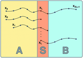
The computation of the correlation function CAB(t) in the ensemble PG[x(τ)] can be performed more efficiently by treating long trajectories as a collection of shorter pathways with shifted starting points. Imagine generating one pathway consisting of 2L + 1 configurations from a starting configuration x in S by propagating L steps in the forward and in the backward direction. From the resulting long trajectory, one can extract a total L + 1 shorter trajectories of length L + 1, one starting in x0, one in x1 and so on up to the trajectory starting at the shooting point xL = x (see Fig. 2). Each of these trajectories contains at least one point in S, namely the shooting point x, and is thus a member of the desired ensemble. Moreover, each of the resulting trajectories is created with the same probability by the algorithm (see eqn (28) in the Appendix), so one can simply average over these pathways by way of the improved algorithm outlined below:
Step 1.
Generate a state x from the probability distribution| |  | (9) |
Step 2.
Starting from x, perform L dynamics steps forward and L steps backward in time. Here, τ = LΔt is the maximum length for which the correlation function CAB(t) is to be computed. In practice, L should be chosen to be sufficiently large such that the system commits to either state A or state B when the trajectory is initiated from a point inside S.
Step 3.
Run over all L + 1 possible trajectories that still envelop the original shooting point xL with the initial points x0,…,xL and compute NS[x(τ)] for each trajectory.
Step 4.
Update the path average appearing in eqn (8) and repeat.
 |
| | Fig. 2 A long pathway consisting of 2L + 1 time-slices (top) can be viewed as the envelope of L + 1 trajectories of length L (below). Note that each of the paths contains at least one configuration in S, namely the original shooting point xL, and is thus a member of the S-ensemble. | |
Once the path average 〈hA(0)hB(t)/NS[x(τ)]〉G has been determined according to this method, it can be combined with the ratio 〈hS〉/〈hA〉, determined from the free energy calculation, to yield the time correlation function CAB(t). The transition rate constant kAB is then obtained from CAB(t) by numerical differentiation (or fit of a straight line) in its linear regime (provided it exists).
3 Results and discussion
3.1 Brownian walker in a double-well
We demonstrate the algorithm by applying it to a simple model for an activated process, namely, a one-dimensional Brownian walker in a double-well potential. For this model, the correlation function 〈hA(0)hB(t)〉S can be computed in a direct simulation, providing a point of comparison to the results of biased and unbiased S-shooting. The system is supposed to obey over-damped Langevin dynamics,| |  | (10) |
where β is the inverse temperature, D is the diffusion constant, F(x) = −dU(x)/dx is the force exerted on the particle by the underlying double-well potentialand ξ is delta-correlated Gaussian white noise with zero mean and unit variance. The chosen parameters are D = 1.0, β = 4.0 and Δt = 0.001. The regions A, S and B are defined as x < −0.4, −0.1 < x < 0.1 and 0.4 < x, respectively (a schematic representation of the chosen region boundaries is shown in Fig. 1c).
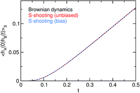
As a reference, we obtain the correlation function 〈hA(0)hB(t)〉S from a single long trajectory produced by a straightforward Brownian dynamics simulation of 5 × 10⁸ time steps. This is done by averaging over all trajectory segments of length τ = 0.5 with at least one point in S. Then, we compute the correlation function 〈hA(0)hB(t)〉S by S-shooting, integrating forward and backward in time from points in S sampled by a Monte Carlo simulation with random displacements drawn from a Gaussian distribution. The whole procedure was repeated by carrying out this Monte Carlo simulation under the influence of a bias Ub = x2/2, thereby obtaining the starting points for biased S-shooting. In terms of averages obtained in the ensemble of trajectories sampled by the algorithm, the correlation function is given by
| |  | (12) |
in the case without bias [see
eqn (32)] and by
| |  | (13) |
in the case with bias [see
eqn (40)].
The agreement between the two variants of S-shooting and the straightforward simulation is shown in Fig. 3 and 4. After an initial transient, the correlation function 〈hA(0)hB(t)〉S enters a linear regime. Consequently, its time derivative exhibits a plateau whose value can be used in the estimate for the reaction rate constant kAB. Using the averages 〈hS〉 = 0.00407 and 〈hA〉 = 0.487 obtained from the straightforward simulation as well as the path average 〈NS[x(τ)]〉S = 24.58, we obtain the rate constant kAB = 0.056.
 |
| | Fig. 3 Correlation function 〈hA(0)hB(t)〉S for a Brownian walker in a double-well potential. The estimates for the correlation function obtained by the S-shooting method (red and blue lines) agree perfectly with the results of the straightforward Brownian dynamics simulation (black line). | |
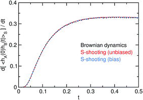 |
| | Fig. 4 Numerical time derivative d〈hA(0)hB(t)〉S/dt of the correlation function. Note the plateau emerging after the initial transient behavior at t ≈ 0.3; this value enters the computation of kAB. | |
Analysis of the convergence of the rate constants as a function of the number of generated pathways indicates that the statistical error in the rate constants obtained by S-shooting is similar to that of divided saddle theory (provided the same method is used for the free energy calculation). Both methods extract the reaction rate constants from the same set of dynamical trajectories such that this equivalence of their efficiencies is not so surprising. Since divided saddle theory has been shown18 to compare well with the reactive flux method of Bennett and Chandler using the effective positive flux approach for the calculation of the transmission coefficient,21 this is the case also for the S-shooting method.
3.2 Cavitation in water under tension
Liquids can sustain remarkably strong tensions due to the free energetic cost associated with the formation of a liquid–vapor interface which impedes an immediate transition to the vapor phase. Water, in particular, can exist in such a metastable state for a long time before decaying into the vapor phase via cavitation, i.e., bubble nucleation, which has implications for the behavior of various biological systems22–26 and for technical applications.27,28 As a further demonstration of S-shooting, we now use it to compute the cavitation rate, i.e., the number of cavitation events per unit time and unit volume, of liquid water at different negative pressures (the cavitation free energy and cavitation rates were first obtained in ref. 29). Specifically, we consider a system of N = 2000 water molecules interacting via the TIP4P/2005 potential30 with long range forces treated with Ewald sums. This system is exposed to pressures ranging from p = −105 MPa to p = −165 MPa at a temperature of T = 296.4 K, where the equation of state is known at moderate negative pressures from experiments.31
To compute the free energy of bubble formation, one must be able to detect bubbles and determine their size for any molecular configuration of this system. This is accomplished using a grid-based procedure that is calibrated to give a thermodynamically consistent estimate for the volume of a bubble.32 The bubble volume obtained in this way corresponds to the average increase in system volume due to the presence of a bubble compared to the unconstrained metastable liquid at the same conditions. We use the volume of the largest bubble present in the system, v, as the reaction coordinate. The free energy, F(ν), as a function of the bubble volume v is given by F(ν) = −ln[ν0p(ν)], where p(ν) is the probability density of encountering a configuration with a largest bubble of size v and ν0 is an arbitrary constant volume required to make the argument of the logarithm dimensionless. We computed p(ν), and from it the free energy F(ν), by employing hybrid Monte Carlo33,34 umbrella sampling35 with “hard” windows in the isobaric–isothermal ensemble.
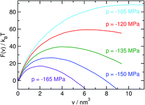
Free energy profiles F(ν) computed for several pressures are shown in Fig. 5. The shape of these curves can be understood in the general framework of classical nucleation theory. The tension applied to the metastable liquid favors the formation and subsequent growth of bubbles through a gain in mechanical work, pν, by expanding the system under tension. This contribution, in conjunction with the free energy cost of forming the interface (Aγ, where A is the surface of the bubble and γ is the surface tension), leads to a barrier in the free energy which separates the metastable liquid from the vapor (shown in Fig. 5). Once the system overcomes this barrier, it transitions to the vapor phase, which, in contrast to the liquid, cannot sustain tension. Consequently, there is no stable basin on the vapor side of the free energy barrier.
 |
| | Fig. 5 Free energy F = −ln[v0p(v)] as a function of the volume v of the largest bubble, where v0 is an arbitrary constant volume, for various pressures. Due to the gain in mechanical work pv associated with the formation of a bubble, the height of the barrier and the size of the critical bubble decrease with increasing tension. Curves are shifted such that the lowest point in the liquid basin aligns for all pressures. | |
In order to apply the S-shooting formalism to the calculation of bubble nucleation rates, we need to define the stable regions A and B as well as the transition region S. Based on the computed free energy profiles, we define the region S to be located around the top of the free barrier and regions A and B left and right of the barrier. A schematic representation of the regions A, B and S employed here is shown in Fig. 1a and a detailed list of the region boundaries is given in Table 1. Once the regions are defined, the averages 〈hA〉 and 〈hS〉 needed for the rate calculation can be determined from the free energy profiles. Next, we need to generate dynamical trajectories from region S in order to compute the correlation function 〈hA(0)hB(t)〉S. Starting from configurations in the region S generated in the free energy calculations, we create pathways by propagating the system backward and forward in time at constant pressure36 and temperature37,38 using a time-reversible integrator.39–41 In order to keep the computational cost manageable, the trajectories used in the rate computation are propagated until they reach a fixed value along the reaction coordinate, rather than for a fixed time. These fixed values were chosen such that they correspond to being approximately 10 kBT lower than the top of the free energy barrier, at which point trajectories are unlikely to re-cross the barrier.† Since this approach leads to trajectories of varying length, trajectories shorter than the desired trajectory length 2L + 1 were padded with their final value on either side of the barrier when computing the correlation function CAB(t).
Table 1 Cavitation rates, J, for various pressures p
|
p/MPa |
A/nm3 |
B/nm3 |
S/nm3 |
1/〈NS〉S |
〈V〉−1〈hS〉/〈hA〉a/nm−3 |
J
/nm−3 ps−1 |
|
The equilibrium probability ratio 〈hS〉/〈hA〉 was obtained from the free energy data shown in Fig. 5 and 〈V〉 is the average volume of the metastable liquid at the appropriate pressure.
The cavitation rate J is obtained by combining the equilibrium probability ratio with a fit to the long-time tail of the time derivative of the correlation function from Fig. 7.
|
| −105 |
ν < 10.3 |
ν > 10.3 |
10.1 < ν < 10.5 |
2.63 × 10⁻³ |
3.77 × 10−40 |
1.98 × 10−41 |
| −120 |
ν < 6.25 |
ν > 6.25 |
6.05 < ν < 6.45 |
2.40 × 10⁻³ |
2.54 × 10⁻²⁷ |
1.05 × 10⁻²⁸ |
| −135 |
ν < 4.075 |
ν > 4.075 |
3.85 < ν < 4.3 |
2.03 × 10⁻³ |
8.92 × 10⁻¹⁹ |
2.81 × 10⁻²⁰ |
| −150 |
ν < 3.06 |
ν > 3.06 |
2.95 < ν < 3.17 |
3.42 × 10⁻³ |
1.30 × 10⁻¹³ |
6.81 × 10⁻¹⁵ |
| −165 |
ν < 2.095 |
ν > 2.095 |
1.985 < ν < 2.205 |
2.89 × 10⁻³ |
2.19 × 10⁻⁹ |
9.75 × 10⁻¹¹ |
Correlation functions 〈hA(0)hB(t)〉S, obtained viaeqn (32) from trajectories in the ensemble PG[x(τ)], are shown in Fig. 6. Since the state S fully overlaps with the adjacent states A and B, one encounters non-finite contributions to the correlation 〈hA(0)hB(t)〉S even for short times, leading to a steep slope for small t (in contrast to the shape of 〈hA(0)hB(t)〉S observed in Section 3.1). Its time derivative, shown in Fig. 7, exhibits transient behavior followed by the emergence of a plateau for longer times. The resulting cavitation rates J = kAB/〈V〉, which span almost 40 orders of magnitude over the investigated range of pressures, are presented in Table 1.
 |
| | Fig. 6 Correlation function 〈hA(0)hB(t)〉S. Note the difference in shape compared to Fig. 3 due to the different boundaries of the states A and B. | |
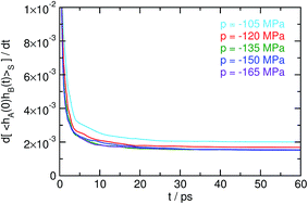 |
| | Fig. 7 Time derivative d〈hA(0)hB(t)〉S/dt of the correlation function depicted in Fig. 6. A fit to the emerging plateau for long times is used in the computation of cavitation rates. | |
4 Conclusion
In the study of rare transitions between long-lived stable states, one often uses large numbers of short molecular dynamics trajectories to determine committors or estimate diffusion coefficients along some collective variable of interest. Here we have presented an algorithm to calculate reaction rate constants by combining dynamical information extracted from such brief trajectories with the results of free energy calculations. For the method to be computationally efficient, the trajectories need to be initiated close to the transition state region such that they have a non-negligible probability to connect the stable states. Hence, the method follows the central idea of the Bennett–Chandler approach,19,20 in which one first computes the transition state theory approximation of the reaction rate constant based on the free energy, and then applies a dynamical correction obtained from short trajectories started on a dividing surface separating the stable states. Our approach uses the same information as the divided saddle theory of Daru and Stirling,18 but processes it in a different way to yield the time correlation function of the stable state populations, from which the reaction rate constant is obtained by taking a time derivative. Knowledge of the correlation function also yields information about the barrier crossing dynamics and permits to verify whether the kinetics follows the exponential behavior expected from the phenomenological rate equations.
Just like the Bennett–Chandler approach and divided saddle theory, the new method, which is equally applicable to under- and overdamped dynamics, also requires a priori knowledge of a reaction coordinate. The reaction coordinate needs to provide an at least rough measure for the progress of the transition and it can be either continuous or discrete, such as the size of the largest crystalline cluster usually used in crystallization studies. As an illustration, we have applied the procedure to a Brownian walker in a double well potential and to cavitation in water at negative pressures, demonstrating that it can be used to determine reaction rate constants in complex condensed environments.
A Derivation of the time correlation function in the S-shooting formalism
A.1 The time correlation function in the S-ensemble
The time correlation function| |  | (14) |
which equals the conditional probability to find the system in B at time t provided it was in A at time 0, can be written as an average in the ensemble P[x(τ)] of trajectories x(τ) of length τ ≥ t:| |  | (15) |
where the notation  indicates a summation over all pathways x(τ), xt is the microscopic state (which we also call configuration or point) of the system at time t, and the probability density of a trajectory consisting of L + 1 configurations is given by
| |  | (16) |
Here, ρ(x0) is the equilibrium probability density of the configuration x0 in the thermodynamic ensemble of interest and p(xi → xi+1) is the probability density of reaching configuration xi+1 when the system in configuration xi is propagated by one step. The time correlation function CAB(t) contains all the information needed to determine the rate constant kAB for transitions from A to B, which is equal to the time derivative of CAB(t) in its linear regime. If transitions from A to B are rare, it is difficult to determine CAB(t) from straightforward molecular dynamics simulations. In the following we present an algorithm to determine CAB(t) that is not affected by this limitation.
Although the integral in eqn (15) extends over all possible trajectories, the non-vanishing contributions to the correlation function CAB(t) stem from trajectories that start in A and reach the product state B by the time t. As such, one can obtain the correlation function CAB(t) by sampling from a constrained ensemble, provided that the constrained ensemble contains all trajectories going from A to B. To define such an ensemble, we introduce the additional region S located such that any trajectory transitioning from A to B necessarily crosses S, i.e., has at least one point in S (see Fig. 1). The correlation function can then be written as
| |  | (17) |
Here, the path function HS[x(τ)] is unity if the trajectory x(τ) has at least one point in S and zero otherwise. We can insert HS[x(τ)] = 1 in the average above without changing the correlation function, because if both hA(0) = 1 and hB(t) = 1 then HS[x(τ)] = 1, and if hA(0) = 0 or hB(t) = 0 the value of HS[x(τ)] does not matter. Multiplying and dividing by 〈HS[x(τ)]〉 one obtains
| |  | (18) |
Here, 〈R〉S = 〈R[x(τ)]HS[x(τ)]〉/〈HS[x(τ)]〉 is the average for an arbitrary path property R[x(τ)] in the ensemble PS[x(τ)] of paths with at least one point in the region S,
| |  | (19) |
where the denominator normalizes the distribution. Since any reactive trajectory,
i.e., any trajectory connecting A and B, has to have points in S, the ensemble
PS[
x(
τ)] contains all reactive trajectories, albeit with a statistical weight that differs from that in the equilibrium trajectory ensemble
P[
x(
τ)] by the factor 〈
HS[
x(
τ)]〉, the probability of an equilibrium trajectory of length
τ to visit S.
In order to evaluate CAB(t) according to eqn (18) using trajectories sampled from PS[x(τ)], we write eqn (18) as
| |  | (20) |
where

is the equilibrium population of the region S, such that the ratio 〈
hS〉/〈
hA〉 can be obtained from the free energy
F(
q) = −
kBT![[thin space (1/6-em)]](https://www.rsc.org/images/entities/char_2009.gif)
ln
![[thin space (1/6-em)]](https://www.rsc.org/images/entities/char_2009.gif) p
p(
q) computed as a function of the reaction coordinate
q. Since 〈
hA(0)
hB(
t)〉
S can be determined as a path average over the ensemble
PS[
x(
τ)], all that is still needed to compute
CAB(
t) is the ratio 〈
HS[
x(
τ)]〉/〈
hS〉. Since the dynamics is microscopically reversible and thus fulfills detailed balance, one can express the average 〈
hS〉 as a path average,
| |  | (21) |
evaluated at an arbitrary point
xi along the trajectories. Since if
hS(
xi) = 1 for at least one point of the trajectory
x(
τ) also
HS[
x(
τ)] = 1, we can insert
HS[
x(
τ)] into the average 〈
hS(
xi)〉 without changing its value and we obtain
| |  | (22) |
But since all configurations xi along a path occur with the same likelihood (see eqn (21)), one can simply average 〈hS(xi)〉S over all L + 1 time slices:
| |  | (23) |
where

is the number of configurations in S. Consequently, 〈
hS〉
S is the fraction of configurations
xi of a given path
x(
τ) located in the region S. Inserting this result into
eqn (20) yields the time-correlation function
CAB(
t) expressed in terms of path averages obtained in the ensemble of trajectories visiting S,
| |  | (24) |
A.2 Relation to the ensemble generated by S-shooting
The algorithm presented in the main text generates trajectories by picking shooting points x in S according to the probability density| |  | (25) |
and subsequently propagating these configurations forward and backward in time. But which ensemble is generated by this algorithm? Since every trajectory x(τ) visiting S, and as such all reactive trajectories, has at least one configuration in S by definition, it can be generated by shooting from points in S. However, in order to verify whether the algorithm generates the desired ensemble, one has to determine how these trajectories are weighted with respect to one another, i.e., one has to inspect the likelihood with which the algorithm generates a particular trajectory. In particular, in doing that one has to take into account that trajectories with multiple points in S have more than one way to be generated by the algorithm.
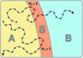
Consider a trajectory  with NS[x(τ)] configurations in region S. (Two examples of such trajectories are shown in Fig. 8.) Here, the NS[x(τ)] subscripts i1,i2,…,iNS[x(τ)] are the indices of the configurations of the trajectory x(τ) that are in S. In the shooting algorithm presented in the main text, the trajectory x(τ) can be generated by shooting from each of these NS[x(τ)] points. Let us now consider the probability density that the trajectory x(τ) is generated from the first one of these points, xi1. For this to happen, configuration xi1 must first be selected from ρS(xi1) and then designated to be the i1-th configuration along the trajectory by drawing the index i1 with probability 1/(L + 1) from the integers 0 to L. Starting from xi1, one then propagates the dynamics for L − i1 steps in the forward and i1 steps in the backward direction using the rules of the underlying dynamics, such that the probability density p[x(τ);xi1] to generate exactly trajectory x(τ) from configuration xi1 is given by
| |  | (26) |
where
![[x with combining macron]](https://www.rsc.org/images/entities/i_char_0078_0304.gif)
is the configuration
x with reversed momenta (because the first product corresponds to propagating the system backward in time). Since the dynamics is microscopically reversible, the transition probability obeys detailed balance; in particular,
| | ρ(xi+1)p(![[x with combining macron]](https://www.rsc.org/images/entities/i_char_0078_0304.gif) i+1 → i+1 → ![[x with combining macron]](https://www.rsc.org/images/entities/i_char_0078_0304.gif) i) = ρ(xi)p(xi → xi+1), i) = ρ(xi)p(xi → xi+1), | (27) |
where we took advantage of the fact that the Hamiltonian does not change when the momenta of a configuration are reversed,
i.e.,
ρ(
![[x with combining macron]](https://www.rsc.org/images/entities/i_char_0078_0304.gif)
) =
ρ(
x). Applying
eqn (27) to
eqn (26) repeatedly, the equilibrium probability density
ρ(
xi1), initially applied to
xi1, is shifted to the first configuration
x0 of the trajectory:
| |  | (28) |
where
hS(
xi1) = 1 since the shooting point
xi1 is in S by construction. The equation above shows that the likelihood of generating
x(
τ) is independent of the chosen shooting point and the probability of generating the trajectory from configuration
xi1 is the same as that of generating it from any of the other possible shooting points
xi2 to

. Hence, the total likelihood to generate a particular trajectory
x(
τ) by shooting from points in S is just
NS[
x(
τ)] times the likelihood of generating it by shooting from one specific point in S:
| |  | (29) |
where we inserted
HS[
x(
τ)] in the first line to emphasize that this algorithm only creates trajectories with at least one configuration in S.
 |
| | Fig. 8 When shooting points are picked from the region S according to the probability density ρS(x), pathways with a larger number NS[x(τ)] of configurations in S are more likely to be created. This overcounting of pathways must be corrected for when computing path averages. | |
The ensemble PG[x(τ)] can be expressed in terms of the ensemble PS[x(τ)] of trajectories visiting S,
| |  | (30) |
Thus, the likelihood to generate a particular trajectory x(τ) in the ensemble PG[x(τ)] generated by the shooting algorithm is related to the likelihood in the ensemble PS[x(τ)] of trajectories visiting S via PG[x(τ)] ∝ NS[x(τ)]PS[x(τ)], i.e., in the ensemble PG[x(τ)], pathways with multiple points in S have a likelihood that is too high compared to the ensemble PS[x(τ)].
Since PG[x(τ)] is normalized [see eqn (22) and (23)], we can now express path averages in the desired ensemble in terms of PG[x(τ)]. The average 〈R[x(τ)]〉S of an arbitrary path property R[x(τ)] is given by
| |  | (31) |
which, by inserting
eqn (30), can be re-written as
| |  | (32) |
Using this expression for averages in the ensemble of pathways visiting S we can rewrite the expression for CAB(t) in eqn (6) in terms of averages in the ensemble PG[x(τ)]:
| |  | (33) |
thus obtaining
eqn (8).
A.3 Biased sampling of shooting points
The computation of the correlation function CAB(t) viaeqn (6) assumes that the starting points of the trajectories are distributed in S according to their Boltzmann weight. Below, we describe how eqn (6) has to be adapted when the initial points are sampled from a biased distribution instead, that is, the shooting points x are generated according towhere the weight b(x) assigned to a configuration due to the bias potential Ub(x) is given by| |  | (35) |
The generation probability p[x(τ);xij] for a path x(τ) by shooting from a specific point xij in S is then given by [see eqn (28)]
| |  | (36) |
As in the previous section, the subscripts i1 to iNS[x(τ)] are the indices of the NS[x(τ)] configurations of the trajectory x(τ) that are in S. Since the path x(τ) can be generated from any configuration in S, the total generation probability of a path with NS[x(τ)] points in S is
| |  | (37) |
where

and the sum runs over all points in S. Since the trajectories are generated by shooting from points located in S, each of the resulting pathways has at least one configuration in S, which allows us to rewrite the equation above as
| |  | (38) |
and, by inserting
eqn (22) and
(23), one obtains
| |  | (39) |
Since we aim to formulate the correlation function CAB(t) in terms of path averages in the ensemble PS[x(τ)], we now express the path average 〈R[x(τ)]〉S in terms of averages calculated in the ensemble PB[x(τ)],
| |  | (40) |
where we divided by

in the second line. Note that since the bias sum
B[
x(
τ)] appears both in the numerator and the denominator, the above expression does not change when the bias is not normalized,
i.e., when

is used for convenience.
Using eqn (40) to rewrite eqn (6), we obtain CAB(t) in terms of biased averages:
| |  | (41) |
When shooting points are obtained from an unbiased distribution, then ![[B with combining tilde]](https://www.rsc.org/images/entities/i_char_0042_0303.gif) [x(τ)] = NS[x(τ)] and eqn (8) is recovered.
[x(τ)] = NS[x(τ)] and eqn (8) is recovered.
Acknowledgements
We thank J. Daru, P. Geiger, and C. Moritz for insightful comments. This work was supported by the Austrian Science Fund (FWF) within the SFB ViCoM [Grant F41] as well as under grant P24681-N20. A. S. also acknowledges support from the Vienna Scientific Cluster (VSC) School. Calculations were carried out on the Vienna Scientific Cluster (VSC).
References
- P. Hänggi, P. Talkner and M. Borkovec, Rev. Mod. Phys., 1990, 62, 251 CrossRef.
-
D. Chandler, in Barrier Crossings: Classical Theory of Rare but Important Events, ed. B. J. Berne, G. Ciccotti and D. F. Coker, Singapore World Sci., 1998, ch. 1, pp. 3–23 Search PubMed.
- A. M. Berezhkovskii and A. Szabo, J. Phys. Chem. B, 2013, 117, 13115–13119 CrossRef CAS PubMed.
- R. B. Best and G. Hummer, Phys. Rev. Lett., 2006, 96, 228104 CrossRef PubMed.
- C. Dellago, P. G. Bolhuis and P. L. Geissler, Adv. Chem. Phys., 2002, 123, 1 CAS.
-
C. Dellago and P. G. Bolhuis, Advanced Computer Simulation Approaches for Soft Matter Sciences III, Springer-Verlag, Berlin, Heidelberg, 2009, vol. 221, p. 167 Search PubMed.
- P. G. Bolhuis and C. Dellago, Eur. Phys. J.: Spec. Top., 2015, 2409 CrossRef CAS.
- A. K. Faradjian and R. Elber, J. Chem. Phys., 2004, 120, 10880–10889 CrossRef CAS PubMed.
- A. Ma and A. R. Dinner, J. Phys. Chem. B, 2005, 109, 6769–6779 CrossRef CAS PubMed.
- W. E, W. Ren and E. Vanden-Eijnden, Chem. Phys. Lett., 2005, 413, 242–247 CrossRef CAS.
- R. B. Best and G. Hummer, Proc. Natl. Acad. Sci. U. S. A., 2005, 102, 6732–6737 CrossRef CAS PubMed.
- P. L. Geissler, C. Dellago and D. Chandler, J. Phys. Chem. B, 1999, 103, 3706 CrossRef CAS.
- W. Lechner, C. Dellago and P. G. Bolhuis, Phys. Rev. Lett., 2011, 106, 085701 CrossRef PubMed.
- B. Peters and B. L. Trout, J. Chem. Phys., 2006, 125, 054108 CrossRef PubMed.
- G. T. Beckham and B. Peters, J. Phys. Chem. Lett., 2011, 2, 1133 CrossRef CAS PubMed.
- S. Jungblut, A. Singraber and C. Dellago, Mol. Phys., 2013, 111, 3527 CrossRef CAS.
- C. Leitold, W. Lechner and C. Dellago, J. Phys.: Condens. Matter, 2015, 27, 194126 CrossRef PubMed.
- J. Daru and A. Stirling, J. Chem. Theory Comput., 2014, 10, 1121–1127 CrossRef CAS PubMed.
-
C. H. Bennett, in Molecular Dynamics and Transition State Theory: The Simulation of Infrequent Events, 1977, ch. 5, pp. 63–97 Search PubMed.
- D. Chandler, J. Chem. Phys., 1978, 68, 2959–2970 CrossRef CAS.
- T. S. van Erp and P. G. Bolhuis, J. Comput. Phys., 2005, 205, 157–181 CrossRef.
- L. Rowland, A. C. L. da Costa, D. R. Galbraith, R. S. Oliveira, O. J. Binks, A. A. R. Oliveira, A. M. Pullen, C. E. Doughty, D. B. Metcalfe, S. S. Vasconcelos, L. V. Ferreira, Y. Malhi, J. Grace, M. Mencuccini and P. Meir, Nature, 2015, 528, 119–122 CAS.
- T. D. Wheeler and A. D. Stroock, Nature, 2008, 455, 208–212 CrossRef CAS PubMed.
- O. Vincent, P. Marmottant, P. A. Quinto-Su and C.-D. Ohl, Phys. Rev. Lett., 2012, 108, 184502 CrossRef PubMed.
- S. N. Patek and R. L. Caldwell, J. Exp. Biol., 2005, 208, 3655–3664 CrossRef CAS PubMed.
- X. Noblin, N. O. Rojas, J. Westbrook, C. Llorens, M. Argentina and J. Dumais, Science, 2012, 335, 1322 CrossRef CAS PubMed.
-
C. E. Brennen, Cavitation and Bubble Dynamics, Oxford University Press, New York, 1995 Search PubMed.
- P. Kumar and R. Saini, Renewable Sustainable Energy Rev., 2010, 14, 374–383 CrossRef.
-
G. Menzl, M. A. Gonzalez, P. Geiger, F. Caupin, J. L. F. Abascal, C. Valeriani and C. Dellago, 2016, arXiv:1606.03392.
- J. L. F. Abascal and C. Vega, J. Chem. Phys., 2005, 123, 234505 CrossRef CAS PubMed.
- K. Davitt, A. Arvengas and F. Caupin, EPL, 2010, 90, 16002 CrossRef.
- M. A. Gonzalez, G. Menzl, J. L. Aragones, P. Geiger, F. Caupin, J. L. F. Abascal, C. Dellago and C. Valeriani, J. Chem. Phys., 2014, 141, 18C511 CrossRef PubMed.
- S. Duane, A. Kennedy, B. Pendleton and D. Roweth, Phys. Lett. B, 1987, 195, 216–222 CrossRef CAS.
- B. Mehlig, D. W. Heermann and B. M. Forrest, Phys. Rev. B: Condens. Matter Mater. Phys., 1992, 45, 679–685 CrossRef.
- G. Torrie and J. Valleau, J. Comput. Phys., 1977, 23, 187–199 CrossRef.
- H. C. Andersen, J. Chem. Phys., 1980, 72, 2384–2393 CrossRef CAS.
- S. Nosé, J. Chem. Phys., 1984, 81, 511 CrossRef.
- W. G. Hoover, Phys. Rev. A: At., Mol., Opt. Phys., 1985, 31, 1695 CrossRef.
- H. Kamberaj, R. Low and M. Neal, J. Chem. Phys., 2005, 122, 224114 CrossRef CAS PubMed.
- T. Miller III, M. Eleftheriou, P. Pattnaik, A. Ndirango, D. Newns and G. Martyna, J. Chem. Phys., 2002, 116, 8649 CrossRef.
- G. Martyna, M. Tuckerman, D. Tobias and M. Klein, Mol. Phys., 1996, 87, 1117–1157 CrossRef CAS.
Footnote |
| † For the two lowest tensions investigated, p = −105 MPa and p = −120 MPa, we extrapolated the free energy to higher bubble volumes to determine the limiting value of the order parameter. |
|
| This journal is © The Royal Society of Chemistry 2016 |
Click here to see how this site uses Cookies. View our privacy policy here.  Open Access Article


![[thin space (1/6-em)]](https://www.rsc.org/images/entities/char_2009.gif) ln
ln![[thin space (1/6-em)]](https://www.rsc.org/images/entities/char_2009.gif) p(q). After initial transient behavior related to the details of the dynamics and the specific definition of the stable states, the time correlation function CAB(t) is expected to enter a linear regime and its time derivative gives the reaction rate constant kAB,
p(q). After initial transient behavior related to the details of the dynamics and the specific definition of the stable states, the time correlation function CAB(t) is expected to enter a linear regime and its time derivative gives the reaction rate constant kAB,

 indicates a summation over all trajectories x(τ) and the path function HS[x(τ)] gives unity if the trajectory x(τ) has at least one configuration in S and zero otherwise. The integral in the denominator on the right-hand side of the equation normalizes the distribution. In the above equation,
  is the probability of a trajectory x(τ) in the unconstrained ensemble of trajectories. In writing this expression, we have assumed that the initial conditions x0 are distributed according to the equilibrium probability density ρ(x0), and that the dynamics are Markovian such that the total path probability can be written as the product of short time transition probabilities p(xi → xi+1). In the ensemble of eqn (5), the path indicator function HS[x(τ)] assigns a vanishing statistical weight to any trajectory x(τ) that has no point in S, thereby restricting the S-ensemble to trajectories visiting S.


 indicates a summation over all pathways x(τ), xt is the microscopic state (which we also call configuration or point) of the system at time t, and the probability density of a trajectory consisting of L + 1 configurations is given by


 is the equilibrium population of the region S, such that the ratio 〈hS〉/〈hA〉 can be obtained from the free energy F(q) = −kBT
![[thin space (1/6-em)]](https://www.rsc.org/images/entities/char_2009.gif) ln
ln![[thin space (1/6-em)]](https://www.rsc.org/images/entities/char_2009.gif) p(q) computed as a function of the reaction coordinate q. Since 〈hA(0)hB(t)〉S can be determined as a path average over the ensemble PS[x(τ)], all that is still needed to compute CAB(t) is the ratio 〈HS[x(τ)]〉/〈hS〉. Since the dynamics is microscopically reversible and thus fulfills detailed balance, one can express the average 〈hS〉 as a path average,
p(q) computed as a function of the reaction coordinate q. Since 〈hA(0)hB(t)〉S can be determined as a path average over the ensemble PS[x(τ)], all that is still needed to compute CAB(t) is the ratio 〈HS[x(τ)]〉/〈hS〉. Since the dynamics is microscopically reversible and thus fulfills detailed balance, one can express the average 〈hS〉 as a path average,


 is the number of configurations in S. Consequently, 〈hS〉S is the fraction of configurations xi of a given path x(τ) located in the region S. Inserting this result into eqn (20) yields the time-correlation function CAB(t) expressed in terms of path averages obtained in the ensemble of trajectories visiting S,

 with NS[x(τ)] configurations in region S. (Two examples of such trajectories are shown in Fig. 8.) Here, the NS[x(τ)] subscripts i1,i2,…,iNS[x(τ)] are the indices of the configurations of the trajectory x(τ) that are in S. In the shooting algorithm presented in the main text, the trajectory x(τ) can be generated by shooting from each of these NS[x(τ)] points. Let us now consider the probability density that the trajectory x(τ) is generated from the first one of these points, xi1. For this to happen, configuration xi1 must first be selected from ρS(xi1) and then designated to be the i1-th configuration along the trajectory by drawing the index i1 with probability 1/(L + 1) from the integers 0 to L. Starting from xi1, one then propagates the dynamics for L − i1 steps in the forward and i1 steps in the backward direction using the rules of the underlying dynamics, such that the probability density p[x(τ);xi1] to generate exactly trajectory x(τ) from configuration xi1 is given by
![[x with combining macron]](https://www.rsc.org/images/entities/i_char_0078_0304.gif) is the configuration x with reversed momenta (because the first product corresponds to propagating the system backward in time). Since the dynamics is microscopically reversible, the transition probability obeys detailed balance; in particular,
is the configuration x with reversed momenta (because the first product corresponds to propagating the system backward in time). Since the dynamics is microscopically reversible, the transition probability obeys detailed balance; in particular,![[x with combining macron]](https://www.rsc.org/images/entities/i_char_0078_0304.gif) i+1 →
i+1 → ![[x with combining macron]](https://www.rsc.org/images/entities/i_char_0078_0304.gif) i) = ρ(xi)p(xi → xi+1),
i) = ρ(xi)p(xi → xi+1),![[x with combining macron]](https://www.rsc.org/images/entities/i_char_0078_0304.gif) ) = ρ(x). Applying eqn (27) to eqn (26) repeatedly, the equilibrium probability density ρ(xi1), initially applied to xi1, is shifted to the first configuration x0 of the trajectory:
) = ρ(x). Applying eqn (27) to eqn (26) repeatedly, the equilibrium probability density ρ(xi1), initially applied to xi1, is shifted to the first configuration x0 of the trajectory:
 . Hence, the total likelihood to generate a particular trajectory x(τ) by shooting from points in S is just NS[x(τ)] times the likelihood of generating it by shooting from one specific point in S:


 and the sum runs over all points in S. Since the trajectories are generated by shooting from points located in S, each of the resulting pathways has at least one configuration in S, which allows us to rewrite the equation above as


 in the second line. Note that since the bias sum B[x(τ)] appears both in the numerator and the denominator, the above expression does not change when the bias is not normalized, i.e., when
  is used for convenience.

![[B with combining tilde]](https://www.rsc.org/images/entities/i_char_0042_0303.gif) [x(τ)] = NS[x(τ)] and eqn (8) is recovered.
[x(τ)] = NS[x(τ)] and eqn (8) is recovered.


