DOI:
10.1039/C5SC03234B
(Edge Article)
Chem. Sci., 2016,
7, 1712-1728
Analytical nuclear gradients for the range-separated many-body dispersion model of noncovalent interactions†
Received
29th August 2015
, Accepted 27th October 2015
First published on 27th October 2015
Abstract
An accurate treatment of the long-range electron correlation energy, including van der Waals (vdW) or dispersion interactions, is essential for describing the structure, dynamics, and function of a wide variety of systems. Among the most accurate models for including dispersion into density functional theory (DFT) is the range-separated many-body dispersion (MBD) method [A. Ambrosetti et al., J. Chem. Phys., 2014, 140, 18A508], in which the correlation energy is modeled at short-range by a semi-local density functional and at long-range by a model system of coupled quantum harmonic oscillators. In this work, we develop analytical gradients of the MBD energy with respect to nuclear coordinates, including all implicit coordinate dependencies arising from the partitioning of the charge density into Hirshfeld effective volumes. To demonstrate the efficiency and accuracy of these MBD gradients for geometry optimizations of systems with intermolecular and intramolecular interactions, we optimized conformers of the benzene dimer and isolated small peptides with aromatic side-chains. We find excellent agreement with the wavefunction theory reference geometries of these systems (at a fraction of the computational cost) and find that MBD consistently outperforms the popular TS and D3(BJ) dispersion corrections. To demonstrate the performance of the MBD model on a larger system with supramolecular interactions, we optimized the C60@C60H28 buckyball catcher host–guest complex. In our analysis, we also find that neglecting the implicit nuclear coordinate dependence arising from the charge density partitioning, as has been done in prior numerical treatments, leads to an unacceptable error in the MBD forces, with relative errors of ∼20% (on average) that can extend well beyond 100%.
1 Introduction
A theoretically sound description of noncovalent interactions, such as hydrogen bonding and van der Waals (vdW) or dispersion forces, is often crucial for an accurate and reliable prediction of the structure, stability, and function of many molecular and condensed-phase systems.1–4 Dispersion interactions are inherently quantum mechanical in nature since they originate from collective non-local electron correlations. Consequently, they pose a significant challenge for electronic structure theory and often require sophisticated wavefunction-based quantum chemistry methodologies for a quantitatively (and in some cases qualitatively) correct treatment. Over the past decade, this challenge has been addressed by a number of approaches seeking to approximately account for dispersion interactions within the hierarchy of exchange–correlation functional approximations in Kohn–Sham density functional theory (DFT),5–53 which is arguably the most successful electronic structure method in widespread use today throughout chemistry, physics, and materials science.54
Based on a summation over generalized interatomic London (C6/R6) dispersion contributions, the class of pairwise-additive dispersion methods provide a simple and computationally efficient avenue for approximately incorporating these ubiquitous long-range interactions within the framework of DFT (see ref. 55 for a recent and comprehensive review of dispersion methods in DFT). Although these pairwise-additive methods are capable of reliably describing the dispersion interactions in many molecular systems, it is now well known that both quantitative and qualitative failures can occur, as demonstrated recently in the binding energetics of host–guest complexes,56 conformational energetics in polypeptide α-helices,57 cohesive properties in molecular crystals,58–60 relative stabilities of (bio)-molecular crystal polymorphs,61–63 and interlayer interaction strengths in layered materials,64,65 to name a few.
In each of these cases, the true many-body nature of dispersion interactions becomes important, whether it is due to beyond-pairwise contributions to the dispersion energy, such as the well-known three-body Axilrod–Teller–Muto (ATM) term,66,67 electrodynamic response screening effects,46,68,69 or the non-additivity of the dynamic polarizability.70 One of the most successful models for incorporating these many-body effects into DFT is the many-body dispersion (MBD) model of Tkatchenko et al.46,47,52,53 which approximates the long-range correlation energy via the zero-point energy of a model system of quantum harmonic oscillators (QHOs) coupled to one another in the dipole approximation. The correlation energy derived from diagonalizing the corresponding Hamiltonian of these QHOs is provably equivalent to the random-phase approximation (RPA) correlation energy in the dipole limit (through the adiabatic-connection fluctuation-dissipation theorem).49,53 The MBD model has consistently provided improved qualitative and quantitative agreement with both experimental results and wavefunction-based benchmarks.46,47Ref. 52 and 69 offer recent perspectives on the role of non-additive dispersion effects in molecular materials and the key successes of the MBD model.
In this work, we seek to extend the applicability of the MBD model by deriving and implementing the analytical gradients of the range-separated many-body dispersion (MBD@rsSCS) energy with respect to nuclear coordinates, thereby enabling efficient geometry optimizations and molecular dynamics simulations at the DFT+MBD level of theory. This paper is principally divided into a theoretical derivation of the analytical forces in the MBD model (Section 2), and a discussion of the first applications of these analytical MBD forces to the optimization of gas-phase molecular systems (Section 4). In Section 2.1–2.2, we start by presenting a self-contained summary of the MBD framework to clarify notation and highlight the different dependencies of the MBD energy on the nuclear coordinates. We then derive analytical nuclear gradients of the MBD@rsSCS correlation energy (Section 2.3). In Section 3 and Section 10 of the accompanying ESI,† we provide computational details. Subsequently, we demonstrate the importance of MBD forces for several representative systems encompassing inter-, intra-, and supra-molecular interactions (Section 4.1–4.3). We finally examine the role of the implicit nuclear coordinate dependence that arises from the partitioning of the electron density into effective atomic volumes (Section 4.4) and conclude with some final remarks on potential avenues for future work.
2 Theory
2.1 Notation employed in this work
As the theory comprising the MBD model has evolved over the past few years, several notational changes have been required to accommodate the development of a more complete formalism that accounts for the various contributions to the long-range correlation energy in molecular systems and condensed-phase materials. In this section, we provide a current and self-contained review of the MBD@rsSCS model followed by a detailed derivation of the corresponding analytical nuclear gradients (forces). Our discussion most closely follows the notation employed in ref. 52 and 53. To assist in the interpretation of these equations, we have also furnished a glossary of symbols utilized in this work as part of the ESI.† For a more thorough discussion of the MBD model (including its approximations and physical interpretations), we refer the reader to the original works46,53 as well as a recent review52 on many-body dispersion interactions in molecules and condensed matter.
Throughout this manuscript, all equations are given in Hartree atomic units (ħ = me = e = 1) with tensor (vector and matrix) quantities denoted by bold typeface. In this regard, one particularly important bold/normal typeface distinction that will arise below is the difference between the 3 × 3 dipole polarizability tensor,
| | 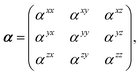 | (1) |
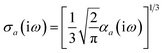
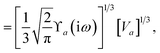
and the “isotropized” dipole polarizability, a scalar quantity obtained
via| |  | (2) |
The Cartesian components of tensor quantities are indicated by superscript Latin indices ij, i.e., Tij is the (i, j)th component of the tensor T. Likewise, Cartesian unit vectors are indicated by {êi, êj}. Atom (or QHO) indices are denoted by subscript Latin indices abc. The index p will be used as a dummy index for summation. The imaginary unit is indicated with blackboard bold typeface, ![[Doublestruck L]](https://www.rsc.org/images/entities/char_e16f.gif) , to distinguish it from the Cartesian component index i. Quantities that arise from the solution of the range-separated self-consistent screening (rsSCS) system of equations introduced by Ambrosetti et al.53 will be denoted by an overline, i.e.,
, to distinguish it from the Cartesian component index i. Quantities that arise from the solution of the range-separated self-consistent screening (rsSCS) system of equations introduced by Ambrosetti et al.53 will be denoted by an overline, i.e.,  . For brevity we will refer to the MBD@rsSCS model (which has also been denoted as MBD* elsewhere) as simply MBD throughout the manuscript.
The MBD model requires keeping track of several different quantities that are naturally denoted with variants of the letter “R”, so we highlight these quantities here for the benefit of the reader. Spatial position, such as the argument of the electron density, ρ(r), is indicated by r. The nuclear position of an atom a (or QHO mapped to that atom) is indicated by  . The internuclear vector is denoted
  , such that the internuclear distance is given by Rab = ||Rab||. It follows that the ith Cartesian component of this internuclear vector is Riab. Finally, the effective vdW radius of an atom a is indicated by
  .
.
The dependence of the long-range MBD correlation energy, EMBD, on the underlying nuclear positions,  will arise both explicitly through the presence of internuclear distance terms, Rab, and implicitly through the presence of effective atomic volume terms,
  , obtained via the Hirshfeld partitioning71 of ρ(r) (see Section 2.2.1). As such, these distinct types of dependence on the nuclear positions will be clearly delineated throughout the review of the MBD model and the derivation of the corresponding MBD nuclear forces below. For notational convenience, we will often use ∂c rather than
  to indicate a derivative with respect to the nuclear position of atom c.
2.2 Review of the many-body dispersion (MBD) model
The MBD formalism is based on a one-to-one mapping of the N atoms comprising a molecular system of interest to a collection of N QHOs centered at the nuclear coordinates, each of which is characterized by a bare isotropic frequency-dependent dipole polarizability, αa(ω). Derived from the electron density, i.e., αa = αa[ρ(r)], these polarizabilities describe the unique local chemical environment surrounding a given atom by accounting for hybridization (coordination number), Pauli repulsion, and other non-trivial exchange–correlation effects (see Section 2.2.1). To account for anisotropy in the local chemical environment as well as collective polarization/depolarization effects, the solution of a range-separated Dyson-like self-consistent screening (rsSCS) equation is used to generate screened isotropic frequency-dependent dipole polarizabilities for each QHO,  (see Section 2.2.2). The MBD model Hamiltonian is then constructed based on these screened frequency-dependent dipole polarizabilities. Diagonalization of this Hamiltonian couples this collection of QHOs within the dipole approximation, yielding a set of interacting QHO eigenmodes with corresponding eigenfrequencies {λ}. The difference between the zero-point energy of these interacting QHO eigenmodes and that of the input non-interacting modes
  , is then used to compute the long-range correlation energy at the MBD level of theory (see Section 2.2.3), i.e.,
| | 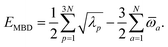 | (3) |
2.2.1 The MBD starting point: bare dipole polarizabilities.
Mapping the N atoms comprising a molecular system of interest onto a collection of N QHOs is accomplished via a Hirshfeld partitioning of ρ(r), the ground state electron density.§Partitioning ρ(r) into N spherical effective atoms enables assignment of the bare frequency-dependent dipole polarizabilities αa(ω) used to characterize a given QHO. Within the MBD formalism, this assignment is given by the following 0/2-order Padé approximant applied to the scalar dipole polarizabilities:73| | 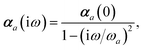 | (4) |
in which αa(0) is the static dipole polarizability and ωa is the characteristic excitation (resonant) frequency for atom a. The dependence of the bare frequency-dependent dipole polarizability in eqn (4) on ρ(r) is introduced by considering the direct proportionality between polarizability and atomic volume,74 an approach that has been very successful in the Tkatchenko–Scheffler (TS) dispersion correction,29i.e.,| | 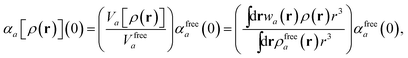 | (5) |
in which Vfreea and αfreea are the volume and static dipole polarizability of the free (isolated) atom in vacuo, respectively, obtained from either experiment or high-level quantum mechanical calculations. Explicit dependence on ρ(r) resides in the effective “atom-in-a-molecule” volume, Va[ρ(r)], obtained via Hirshfeld partitioning71 of ρ(r) into atomic components, in which the weight functions,| | 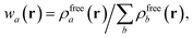 | (6) |
are constructed from the set of spherical free atom densities, {ρfreeb(r)}. At present, we compute the Hirshfeld partitioning and subsequently the MBD energy and forces as an a posteriori update to the solution of the non-linear Kohn–Sham equations, i.e., without performing self-consistent updates to ρ(r). Future work will address the impacts of computing the Hirshfeld partitioning iteratively75 and using the MBD potential to update the Kohn–Sham density self-consistently. In this regard, recent work on the self-consistent application of the TS method indicates that self-consistency can have a surprisingly large impact on the charge densities, and corresponding work functions, of metallic surfaces,76 so we anticipate that self-consistent MBD will be particularly interesting for the study of surfaces and polarizable low-dimensional systems.
For later convenience, we rewrite eqn (4) and (5) to collect all quantities that do not implicitly depend on the nuclear coordinates through Va[ρ(r)] into the quantity ϒa(ω):
| |  | (7) |
| | | ≡ ϒa(ω)Va[ρ(r)]. | (8) |
2.2.2 Range-separated self-consistent screening (rsSCS).
Let A be a 3N × 3N block diagonal matrix formed from the frequency-dependent polarizabilities in eqn (7):¶| |  | (9) |
This quantity will be referred to as the bare system dipole polarizability tensor. For a given frequency, range-separated self-consistent screening (rsSCS) of A(ω) is then accomplished by solving the following matrix equation52,77 (see the ESI† for the detailed derivation of eqn (11)):| | 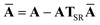 | (10) |
| |  | (11) |
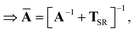
where TSR is the short-range dipole–dipole interaction tensor, defined below in Section 2.2.4 eqn (35). The matrix  is the (dense) screened non-local polarizability matrix, sometimes called the relay matrix.||
Partial internal contraction over atomic sub-blocks of  yields the screened and anisotropic atomic polarizability tensors (the corresponding molecular polarizability is obtained by total internal contraction), i.e.,
| |  | (12) |
The static “isotropized” screened polarizability scalars,

, that appear in the MBD Hamiltonian in
eqn (17) and Section 2.2.3 below are then calculated from
 via
via| | 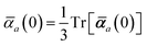 | (13) |
as described above in
eqn (2). Note that
eqn (11) and
(12) can be solved at any imaginary frequency,
ω, so we do not require the Padé approximant given in
eqn (4) to bootstrap from

to

. However, the relationship between

and

, given in
eqn (15), is one that is derived from the Padé approximant for the bare polarizability
α(
ω).
In the non-retarded regime, the Casimir–Polder integral relates the effective C6,ab dispersion coefficient to the dipole polarizabilities of QHOs a and b via the following integral over imaginary frequencies:78
| | 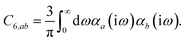 | (14) |
By solving
eqn (11) and
(12) on a grid of imaginary frequencies {
yp}, a set of screened effective
C6 coefficients,

, can be determined by a Gauss–Legendre quadrature estimate of the integral in
eqn (14). The screened QHO characteristic excitation frequency,

, is then calculated as
| | 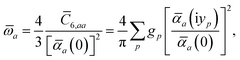 | (15) |
where
gp and
yp are the quadrature weights and abscissae, respectively. Scaling of the usual Gauss–Legendre abscissae from [−1, 1] to the semi-infinite interval [0, ∞) is discussed in the accompanying ESI.
†
2.2.3 The MBD model Hamiltonian.
The central concept in the MBD model is the Hamiltonian for a set of coupled QHOs that each fluctuate within an isotropic harmonic potential  , and acquire instantaneous dipole moments, da = qaxa, that are proportional to the displacement, xa, from the equilibrium position and charge, qa, on each oscillator. This Hamiltonian defines the so-called coupled fluctuating dipole model (CFDM),79 and is given by:
| |  | (16) |
where Tab is the dipole–dipole interaction tensor that couples dipoles a and b.
In the range-separated MBD model,53T is replaced by a long-range screened interaction tensor,  (as defined in Section 2.2.4 and eqn (37) below), and the fluctuating point dipoles are replaced with the Gaussian charge densities of QHOs, with effective masses
  obtained from their respective static polarizabilities and excitation frequencies. The corresponding range-separated MBD model Hamiltonian is therefore:53
| | 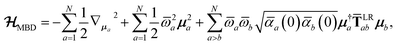 | (17) |
in which

is the mass-weighted dipole moment of QHO
a that has been displaced by
ξa from its equilibrium position.
** The first two terms in
eqn (17) represent the kinetic and potential energy of the individual QHOs, respectively, and the third term is the two-body coupling due to the long-range dipole–dipole interaction tensor,

, defined below in
eqn (37).
By considering the single-particle potential energy and dipole–dipole interaction terms in eqn (17), we can construct the 3N × 3N MBD interaction matrix, which is comprised of 3 × 3 subblocks describing the coupling of each pair of QHOs a and b:
| | 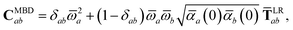 | (18) |
where
δab is the Kronecker delta between atomic indices.
The eigenvalues {λp} obtained by diagonalizing CMBD correspond to the interacting (or “dressed”) QHO modes, while  correspond to the modes of the non-interacting reference system of screened oscillators. The MBD correlation energy is then evaluated viaeqn (3) as the zero-point energetic difference between the interacting and non-interacting modes.
For periodic systems, all instances of the dipole–dipole interaction tensor would be replaced by
| |  | (19) |
where the sum over
b′ indicates a lattice sum over the periodic images of atom
b. Since this is an additive modification of
T, it will not qualitatively modify the expressions for the analytical nuclear derivatives of the MBD energy. Hence, the derivation of the nuclear forces presented herein (and the accompanying chemical applications) will focus on non-periodic (or isolated) systems. We note in passing that the current implementation of the MBD energy and nuclear forces in QUANTUM ESPRESSO (QE)
80 is able to treat both periodic and non-periodic systems. In this regard, a forthcoming paper
81 will describe the details of the implementation and discuss the subtleties required to make the computation of well-converged MBD nuclear forces efficient for periodic systems.
2.2.4 The range-separated dipole–dipole interaction.
Prior to range-separation, the 3 × 3 sub-block Tab of the dipole–dipole interaction tensor T, which describes the coupling between QHOs a and b, is defined as:| |  | (20) |
where νab is the frequency-dependent Coulomb interaction between two spherical Gaussian charge distributions.82 This frequency-dependent interaction arises due to the fact that the ground state of a QHO has a Gaussian charge density:| |  | (21) |
where  ,
,| |  | (22) |
and| |  | (23) |
is the effective correlation length of the interaction potential defined by the widths of the QHO Gaussians (see eqn (24) below). As such, the dependence of T on both the frequency and (implicitly) on the nuclear coordinates originates from ∑ab(ω) (see also eqn (7) and (8)).
In terms of the bare dipole polarizability, the width of the QHO ground-state Gaussian charge density is given by:
| |  | (24) |
| |  | (25) |
where
is the “isotropized”
bare dipole polarizability and
eqn (8) was used to make the effective volume dependence more explicit.
The Cartesian components of the dipole–dipole interaction tensor in eqn (20) (with all QHO indices and frequency-dependence of ζ suppressed) are given by:
| | 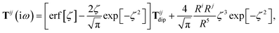 | (26) |
where
Ri =
Rab·
êi is the
ith Cartesian component of
Rab, and
Tdip is the frequency-
independent interaction between two point dipoles:
| |  | (27) |
with
δij indicating the Kronecker delta between Cartesian indices.
The range-separation of the dipole–dipole interaction tensor is accomplished by using a Fermi-type damping function,18,24,29
| | f![[thin space (1/6-em)]](https://www.rsc.org/images/entities/char_2009.gif) (Zab) = [1 + exp[−Zab]]−1, (Zab) = [1 + exp[−Zab]]−1, | (28) |
which depends on
Zab, the ratio between
Rab, the internuclear distance, and
Sab, the scaled sum of the effective vdW radii of atoms
a and
b,
:
| |  | (29) |
| |  | (30) |
Here, the range-separation parameter
β is fit once for a given exchange–correlation functional by minimizing the energy deviations with respect to highly accurate reference data.
53 The short- and long-range components of the dipole–dipole interaction tensor in
eqn (26) are then separated according to:
| | | TSR = [1 − f(Z)]T | (31) |
and
| | | TLR = f(Z)T. | (32) |
However, at long-range, the frequency-dependence in
T dies off quickly, so when evaluating the MBD Hamiltonian we replace
eqn (32) with the approximation
| | | TLR ≃ f(Z)Tdip | (33) |
which is equivalent to taking erf
[
ζ] ≃ 1 and exp
[−
ζ2] ≃ 0 in
eqn (26) and
(32). This has the added benefit of improved computational efficiency since special functions such as the error function and exponential are relatively costly to compute. As shown in Fig. S1 in the ESI,
† these approximations are exact to within machine precision for
ζ > 6, and thus in practice by the time
f(
Z) has obtained a substantial value, the frequency dependence in
T has vanished, thereby justifying
eqn (33).
The rsSCS procedure described in Section 2.2.2 adds a further subtlety in that it modifies the effective vdW radii in the definition of the Sab and Zab quantities above (see ref. 46 and 52 for a more detailed discussion of these definitions). For the short-range interaction tensor (i.e., the tensor used in the rsSCS procedure) the damping function utilizes effective vdW radii calculated at the Tkatchenko–Scheffler (TS) level:29
| |  | (34) |
where

is the free-atom vdW radius defined in
ref. 29 using an electron density contour, not the Bondi
83 radius that corresponds to the “atom-in-a-molecule” analog of this quantity. To indicate that the TS-level effective vdW radii are being used, the argument of the damping function for the short-range interaction tensor, used in
eqn (10) and
(11), will be denoted with
ZTS (
cf.eqn (29),
(30) and
(34)):
| | | TSR = [1 − f(ZTS)]T. | (35) |
For the long-range dipole–dipole interaction tensor used in the MBD Hamiltonian in
eqn (17), the damping function utilizes the self-consistently screened effective vdW radii:
46| |  | (36) |
wherein the ratio

takes the place of
V/
Vfree thereby still exploiting the proportionality between polarizability and volume.
52,74 To indicate that the screened effective vdW radii are being used, the argument of the damping function for the long-range interaction tensor will be denoted with

(
cf.eqn (29),
(30) and
(36)):
| |  | (37) |
This dependence on

is why we use an overline on
TLR above, and in
eqn (17) and
(18).
2.3 Derivation of the MBD nuclear forces
With the above definitions in hand, we are now ready to proceed with the derivation of the analytical derivatives of the MBD correlation energy with respect to the nuclear (or ionic) position  of an arbitrary atom c.††
These MBD forces are added to the DFT-based forces. As mentioned above in Section 2.1, two distinct types of nuclear coordinate dependence will arise: explicit dependence through  and implicit dependence through
  (as moving a neighboring atom c will slightly alter the effective volume assigned to atom a). Future work will address the effects of the MBD contribution to the exchange–correlation potential when applied self-consistently, which will ultimately impact ρ(r). Our current work neglects these effects, and computes MBD as an a posteriori correction to DFT, i.e., non-self-consistently.
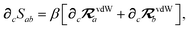
Having carefully separated out the implicit dependence on  in the relevant quantities above, the derivation proceeds largely by brute force application of the chain and product rules. The derivative of the MBD correlation energy given in eqn (3) is governed by:
| |  | (38) |
hence requiring derivatives of the screened excitation frequencies,

, as well as the eigenvalues,
λp, of the
CMBD matrix. Since
CMBD is real and symmetric, it has 3
N orthogonal eigenvectors. We therefore do not concern ourselves here with repeated eigenvalues (see the ESI
† for a more detailed discussion) and take derivatives of
λp as:
87| |  | (39) |
| |  | (40) |
| |  | (41) |
where
χ is the matrix of eigenvectors of
CMBD and
Λ = diag[
λp] is the diagonal matrix of eigenvalues. To evaluate this last line we require the derivative of the
ab block of
CMBD (
cf.eqn (18)),
| |  | (42) |
To proceed any further we now need the derivatives of

,

, and

. From
eqn (15), we find that the derivative of the screened excitation frequency,

, requires us to evaluate derivatives of

(with

as a specific case) as follows:
| |  | (43) |
The derivative of the screened polarizability,

,
eqn (13), is calculated from the “isotropized” partial contraction of

(with the frequency dependence suppressed):
| |  | (44) |
Using
eqn (11) and
(35) and expanding the derivative of the inverse of a non-singular matrix, we have
| |  | (45) |
Using
eqn (8) and
(9), we compute
∂cA as:
| |  | (46) |
In
eqn (46) we have terminated the chain-rule with
∂cVa, which has remaining
implicit dependence on the nuclear coordinates. We regard
∂cVa as one of our three fundamental derivatives since the Hirshfeld partitioning is typically computed separately from the rest of the MBD algorithm. Discussion of how to compute
∂cVa may be found in the ESI.
†
In considering the derivatives of the dipole–dipole interaction tensors, we will encounter both implicit and explicit nuclear position dependence through ζabviaeqn (22). The derivatives of TSR, eqn (35), and  , eqn (37), are fairly complicated, so it will help to consider first the damping function, f, in isolation. Here,
| |  | (47) |
| |  | (48) |
| |  | (49) |
where
∂cRab is calculated as
| | 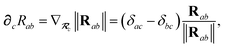 | (50) |
and the effective vdW radii have only implicit nuclear coordinate dependence. For the gradient of
TSR,
eqn (35), we require the derivative of the TS-level effective vdW radii,
eqn (34):
| | 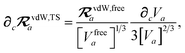 | (51) |
while for the gradient of

,
eqn (37), we require the derivative of the screened effective vdW radii,
eqn (36):
| | 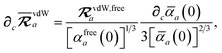 | (52) |
which was evaluated using
eqn (44)–(46).
In the following we suppress the QHO indices (a, b, c) where possible so that the Cartesian indices (i, j) are highlighted. First we consider the derivative of Tdip, eqn (27), which is given by:
| | 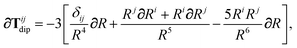 | (53) |
where
∂Ri is evaluated as:
| |  | (54) |
Since the long-range dipole–dipole interaction tensor is approximated with the frequency-independent
Tdip (thereby eliminating
ζ),
eqn (47)–(53) provide us with all of the quantities needed to evaluate

as:
| |  | (55) |
The derivative of
TSR is more complex since
T depends on
ζ:
| | | ∂cTijab,SR = −Tijab∂cf(ZTSab) + [1 − f(ZTSab)]∂cTijab, | (56) |
in which the derivative of
Tij is given below (see the ESI
† for a detailed derivation):
| |  | (57) |
wherein we have defined the following function for compactness,
| |  | (58) |
The derivative of ζ
ab is given by (with QHO indices restored to express
∂c∑
ab from
eqn (23)):
| |  | (59) |
where
∂cσa is computed from
eqn (25) as
| |  | (60) |
We have now reduced the analytical nuclear derivative of the MBD correlation energy to quantities that depend on three fundamental derivatives: ∂cRab, ∂cRiab and ∂cVa. The expressions for ∂cRab and ∂cRiab have been given above in eqn (50) and (54), and are straightforward to implement. The computation of ∂cVa is outlined briefly in the ESI.†
3 Computational details
We have implemented the MBD energy and analytical nuclear gradients (forces) in a development version of Quantum ESPRESSO v5.1 (QE).80 A forthcoming publication will discuss the details of this implementation, including the parallelization and algorithmic strategies required to make the method efficient for treating large-scale condensed-phase systems.81
All calculations were performed with the Perdew, Burke, and Ernzerhof (PBE) exchange–correlation functional,88,89 and Hamann–Schlueter–Chiang–Vanderbilt (HSCV) norm-conserving pseudopotentials.90–92 As a point of completeness, it should be noted that in QE the Hirshfeld partitioning has only been implemented for norm-conserving pseudopotentials, and thus the MBD method cannot presently be used with ultrasoft pseudopotentials or projector-augmented wave methods. To ensure a fair comparison with our implementation of the MBD model, all TS calculations were performed as a posteriori corrections to the solution of the non-linear Kohn–Sham equations, i.e. we turned off the self-consistent density updates from TS. Additional computational details, including detailed convergence tolerances and basis sets are given in Section 10 of the ESI.† For comparison with the D3(BJ) dispersion correction of Grimme et al.35,45 (hereafter abbreviated as D3) we also optimized structures using ORCA v3.03.93 We used the atom-pairwise version of D3(BJ) since only numerical gradients were available for the three-body term.
4 Results and discussion
To verify our implementation of the MBD energy in QE, we compared against the implementation of the MBD@rsSCS model in the FHI-aims code94,95 and find agreement to within 10−11Eh. We next verified our implementation of the analytical gradients by computing numerical derivatives via the central difference formula and find agreement within the level of expected error given the finite spacing between the grid points describing ρ(r) and error propagation of finite differences of the Hirshfeld effective volume derivatives.
To demonstrate the efficiency and accuracy of the analytical MBD nuclear gradient, we performed geometry optimizations on representative systems for intermolecular interactions (benzene dimer), intramolecular interactions (polypeptide secondary structure), and supramolecular interactions (buckyball catcher host–guest complex). We subsequently examined the importance of the implicit nuclear coordinate dependence that arises from the Hirshfeld effective volume gradient ∂V in the computation of the MBD forces.
4.1 Intermolecular interactions: stationary points on the benzene dimer potential energy surface
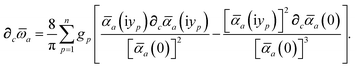
As the prototypical example of the π–π interaction, there have been a large number of theoretical studies on the benzene dimer using very high-level wavefunction theory methods.96–117 Since the intermolecular attraction between the benzene dimer arises primarily from a balance between dispersion interactions and quadrupole–quadrupole interactions (depending on the intermolecular binding motif), the interaction energy is quite small (∼2–3 kcal mol−1) and the potential energy surface (PES) is very flat. Consequently, resolving the stationary points of this PES is quite challenging for both theory and experiment. The prediction of the interaction energy in the benzene dimer represents a stringent test of the ability of a given electronic structure theory method to capture and accurately describe non-bonded intermolecular interactions. Historically, three conformers of the dimer have received the most attention, namely the “sandwich,” “parallel-displaced,” and “T-shaped” structures. Using the high-level benchmark interaction energy calculations as a guide, several studies have used a variety of more approximate methods to examine the PES more broadly.107,109,115,117 By scanning the PES of the benzene dimer with DFT-based symmetry adapted perturbation theory (DFT-SAPT), Podeszwa et al.107 identified 10 stationary points, i.e., either minima (M) or saddle points (S) of the interaction energy (see Fig. 1). Most wavefunction studies of the benzene dimer PES have used a fixed monomer geometry, assuming that the weak interactions will produce very little relaxation of the rigid monomer.104 Using the highly accurate fixed benzene monomer geometry of Gauss and Stanton,102 Bludský et al.113 performed counterpoise-corrected geometry optimizations of these 10 configurations at the PBE/CCSD(T) level of theory, with an aug-cc-pVDZ basis set. The resulting geometries are among the largest molecular dimers to be optimized with a CCSD(T) correction to date and represent the most accurate available structures for the dimer of this classic aromatic system.
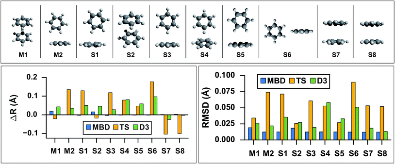 |
| | Fig. 1
Top: graphical depictions of the 10 configurations that correspond to stationary points on the benzene dimer PES, following the nomenclature of Podeszwa et al.107 (Mn = minima; Sn = saddle points). Left: Change in inter-monomer distance, R, relative to the PBE/CCSD(T) reference for geometries optimized with PBE+vdW methods: MBD (shown in blue), TS (shown in yellow) and D3 (shown in green). PBE+MBD consistently predicts the correct inter-monomer distance. For the stacked configurations (M1, S2, S7, and S8) PBE+TS shortens the inter-monomer distance, while for T-shaped configurations (M2, S1, S3, S4, S5, and S6) the inter-monomer distance is elongated. For all configurations except the sandwich-stacked S7 and S8 structures, PBE+D3 overestimates the inter-monomer distance. Right: Root-mean-square-deviations (RMSD) in Å between the PBE+vdW and PBE/CCSD(T)107 optimized geometries of these 10 benzene dimer configurations. The RMSD between the PBE+MBD and reference PBE/CCSD(T) geometries (shown in blue) are uniformly small and consistent across all minima and saddle points on the benzene dimer PES. For several Mn and Sn configurations, the PBE+D3 optimized geometries (shown in green) agree quite well with the PBE/CCSD(T) reference, while the PBE+TS optimized geometries (shown in yellow) have more significant deviations. | |
As a first application of the MBD analytical nuclear gradients derived and implemented in this work, we performed geometry optimizations on these 10 benzene dimer configurations at the PBE+MBD, PBE+TS, and PBE+D3 levels of theory. All of the geometry optimizations performed herein minimized the force components on all atomic degrees of freedom according to the thresholds and convergence criteria specified in Section 10 of the ESI† (i.e., frozen benzene monomers were not employed in these geometry optimizations). The root-mean-square-deviations (RMSD in Å) between the PBE+MBD, PBE+TS, and PBE+D3 optimized geometries with respect to the reference PBE/CCSD(T) results are depicted in Fig. 1.
From this figure, it is clear that the PBE+MBD method, with a mean RMSD value of 0.01 Å (and a vanishingly small standard deviation of 3 × 10⁻⁴ Å) with respect to the reference PBE/CCSD(T) results, was able to provide uniformly accurate predictions for the geometries of all of the benzene dimer configurations considered. These findings are encouraging and consistent with the fact that the PBE+MBD method yields significantly improved binding energies for the benzene dimer as well as a more accurate quantitative description of the fractional anisotropy in the static dipole polarizability of the benzene monomer.52 This is also consistent with the finding of von Lilienfeld and Tkatchenko that the three-body ATM term contributes ∼25% of the binding energy of the benzene dimer in the parallel displaced configuration.118
With a mean RMSD value of 0.03 ± 0.01 Å and 0.05 ± 0.02 Å respectively, the PBE+D3 and PBE+TS methods both yielded a less quantitative measure of the benzene dimer geometries with respect to the reference PBE/CCSD(T) data. Of the 7 benzene dimer configurations for which the PBE+TS RMSD values were greater than 0.05 Å (namely M2, S1, S3, S4, S6, S7, and S8), it is difficult to identify a shared intermolecular binding motif among them. Interestingly, PBE+D3 seems to fare better on sandwich-stacked geometries and it is only the T-shaped S4 and S6 which have RMSDs above 0.05 Å.
However, analysis of the inter-monomer distance (see Fig. 1) reveals that PBE+TS tends to shorten the inter-monomer distance, R, for stacked geometries (M1, S2, S7, and S8) by an average of 0.03 Å relative to the PBE/CCSD(T) results, while it elongates the inter-monomer distance by an average of 0.09 Å for T-shaped structures.
We believe that these observations can be explained by the fact that the frequency-dependent dipole polarizability (FDP) in the TS model is approximated by an isotropic scalar instead of an anisotropic tensor quantity. A consequence of this approximation is that the in-plane components of the FDP in the benzene monomer are underestimated while the out-of-plane component is overestimated. In the stacked benzene dimer configurations, the inter-monomer distances are primarily determined by the coupling of the induced dipole moment in the direction of the out-of-plane component of one monomer with the induced dipole moment in the direction of the out-of-plane component of the other monomer. As such, the interaction along the inter-monomer axis, R, is overestimated, which leads to TS predicting an inter-monomer distance that is too short with respect to the available reference data. This effect is more apparent in the sandwich-stacked configurations (S7 and S8) than the parallel-displaced-stacked configurations (M1 and S2), which is also consistent with the fact that the argument above would affect configurations in which the monomers are directly aligned (i.e., have a rise and no run) to a much larger degree than those that are displaced (i.e., have a rise and a run). For the T-shaped configurations, the situation is slightly more complicated (and less clear than in the stacked cases). Here, the intermolecular binding motif balances several components, e.g., the out-of-plane component on one monomer with the in-plane component of the other monomer. From Fig. 1, we also observed that D3, like TS, shortens the inter-monomer distance for both S7 and S8. However, PBE+D3 elongates the inter-monomer distance by an average of 0.06 Å for all other dimer geometries.
For both stacked and T-shaped structures, PBE+MBD performs much more consistently, elongating the inter-monomer distance by a scant 5 × 10⁻³ Å and 1 × 10⁻³ Å for stacked and T-shaped configurations, respectively. This is believed to be because PBE+MBD captures the anisotropy (and screening) in the FDP of the benzene monomer. The MBD model essentially fixes the issues with TS described above and is able to yield consistent results for all inter-monomer binding motifs of the benzene dimer. In the MBD case, the beyond-pairwise dispersion interactions might also play a role here, but their effect is harder to estimate without explicitly calculating the decomposition of the MBD energy and forces into individual n-body terms (n = 2, 3,…, N).
We note that RMSD values in the range of 0.03–0.08 Å, and errors on the inter-monomer distances of 0.05–0.15 Å, in the geometries of small molecular dimers (as found here with the PBE+TS and PBE+D3 methods) are not unacceptably large in magnitude; however, these differences will become even more pronounced as the sizes and polarizabilities of the monomers continue to increase.47,52,61,69 In this regime, the MBD method—by accounting for both anisotropy and non-additivity in the polarizabilities as well as beyond-pairwise many-body contributions to the long-range correlation energy—is expected to yield accurate and consistent equilibrium geometries for such systems. As such, the combination of DFT+MBD has the potential to emerge as a computationally efficient and accurate electronic structure theory methodology for performing scans of high-dimensional PESs for molecular systems whose overall stability is primarily dictated by long-range intermolecular interactions.
4.2 Intramolecular interactions: secondary structure of polypeptides
As a second application, we considered the intramolecular interactions that are responsible for the secondary structure in small polypeptide conformations. In particular, we studied 76 conformers of 5 isolated polypeptide sequences (GFA, FGG, GGF, WG, and WGG), which are comprised of the following four amino acids: glycine (G), alanine (A), phenylalanine (F), and tryptophan (W). This set of peptide building blocks includes the simplest amino acids, glycine and alanine (with hydrogen and methyl side chains, respectively), as well as the larger aromatic amino acids, phenylalanine and tryptophan (with benzyl and indole side chains, respectively). Although each of these polypeptides are relatively small (with 34–41 atoms each), a significant amount of conformational flexibility is present due to the non-trivial intramolecular binding motifs found in these systems, such as non-bonded side chain–backbone interactions and intramolecular hydrogen bonding. In fact, it is the presence of these interactions that leads to the formation of α-helices and β-pleated sheets—the main signatures of secondary structure in large polypeptides and proteins.
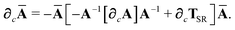
Following a benchmark study by Valdes et al.,119 in which the geometries of these 76 conformers were optimized using second-order Møller–Plesset perturbation theory120 (MP2) within the resolution-of-the-identity approximation121–123 (RI-MP2) and the fairly high-quality cc-pVTZ atomic orbital basis set,124 we performed geometry optimizations on this set of conformers with several vdW-inclusive DFT approaches, namely, PBE+D3, PBE+TS, and PBE+MBD. All of the geometry optimizations performed in this section minimized the force components on all atomic degrees of freedom according to the thresholds and convergence criteria specified in Section 10 of the ESI.† Treating the MP2 geometries as our reference, Fig. 2 displays box-and-whisker plots of the distributions of root-mean-square deviations (in Å) obtained from geometry optimizations employing the aforementioned vdW-inclusive DFT methodologies.
 |
| | Fig. 2 Box-and-whisker plots showing the distribution of root-mean-square-deviations (RMSDs) in Å between 76 conformers of 5 isolated small peptides optimized with PBE+MBD (blue), PBE+TS (yellow) and PBE+D3 (green) compared against the MP2 reference geometries of ref. 119. Whiskers extend to data within 1.5 times the interquartile range.125 PBE+MBD consistently yields optimized geometries closer to the MP2 reference than either PBE+D3 or PBE+TS. Median (maximum) values are: 0.06 (0.28) Å for PBE+MBD, 0.09 (0.52) Å for PBE+TS, and 0.14 (1.10) Å for PBE+D3. | |
Here we find that the PBE+MBD method again yields equilibrium geometries that are consistently in closer agreement with the reference MP2 data than both the PBE+TS and PBE+D3 methodologies. For instance, the RMSDs between the PBE+MBD and MP2 conformers are smaller than 0.12 Å for all but one GGF conformer (34: GGF04), with an overall mean RMSD value of 0.07 ± 0.03 Å. In contrast to the intermolecular case of the benzene dimer, the PBE+TS method performs significantly better than PBE+D3 on the same benchmark set of polypeptides, with overall mean RMSD values of 0.11 ± 0.07 Å and 0.20 ± 0.17 Å, respectively. In this regard, the whiskers in Fig. 2 extend to RMSD values that are within 1.5 times the interquartile range (i.e., following the original, although arbitrary, convention for determining outliers suggested by Tukey125), which highlights the fact that there are several conformers for which both PBE+TS and PBE+D3 predict equilibrium geometries that are significantly different than MP2.
Although MP2 is the most economical wavefunction-based electronic structure method that can describe dispersion interactions, MP2 does not properly account for long-range many-body effects and tends to grossly overestimate C6 dispersion coefficients,126 which in general leads to an overestimation of the binding energies of dispersion-bound complexes such as the benzene dimer. Since PBE+MBD should in general bind less strongly than MP2, we expect the side-chain-to-backbone distance to elongate slightly for bent conformers. In the same breath, conformers in which the side chain is extended away from the backbone are expected to show less deviation between MP2 and PBE+MBD as the side-chain-to-backbone dispersion interaction will be less significant in determining the overall geometry of the conformer.
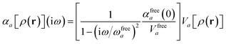
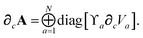
Aside from the noticeable outliers, the structural deviations in most of the conformers correspond to small rotations or deflections of terminal groups and side chains due to dispersion-based interactions, in contrast to the backbone which is constrained by non-rotatable bonds. In Fig. 3 we present representative overlays of this rearrangement, showing the MP2 (blue), PBE+MBD (red), and PBE+D3 (yellow) geometries. In (a) structure 17 (GFA03) is a conformer for which both PBE+MBD and PBE+D3 give small/moderate RMSDs with MP2. Both PBE+MBD and PBE+D3 open the cleft between the alanine and phenylalanine, also causing the amine on the backbone to slightly rotate. The relative positioning of these structures is expected, given the tendency of MP2 to over-bind dispersion interactions and the tendency of PBE+D3 to under-bind. In (b) structure 48 (WG03), again shows PBE+MBD agreeing well with MP2, but slightly opening the backbone-side chain distance. However, PBE+D3 performs unfavorably on this structure, yielding an RMSD of 1.10 Å, due to large rotations in both the backbone and indole side-chain.
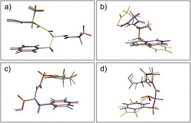 |
| | Fig. 3 Overlays of the structures obtained from geometry optimization with MP2 (blue), PBE+MBD (red), and PBE+D3 (yellow). In both (a) GFA03 and (b) WG03, the MBD correction opens the cleft between the backbone and aromatic side-chain as MP2 tends to over-bind dispersion interactions. (c) In GGF04, PBE+MBD rotates the phenylalanine and alanine groups together. (d) In FGG215, since the side-chain is farther away from the backbone, PBE+MBD matches the MP2 geometry almost exactly. | |
Structures where the side-chain lies farther off to the side of the backbone, such as 4 (FGG215) shown in panel (d), show the smallest RMSDs between the PBE+MBD and reference MP2 geometries with the PBE+MBD geometry lying almost exactly on top of the MP2 geometry. However, FGG215 is again a structure where D3 does poorly with respect to the MP2 geometry, this time rotating the benzyl side-chain away from the terminal glycine, yielding an RMSD of 0.64 Å.
The structure for which the PBE+MBD method has the largest RMSD, at 0.28 Å, is 34 (GGF04), shown in panel (c). As opposed to opening a cleft like in GFA03, PBE+MBD rotates the phenylalanine and alanine groups together. This rotation occurs because the terminal hydrogen on the glycine is attracted to the π-system on the phenylalanine. The rigid nature of the glycine combined with the rotatable bond in the phenylalanine, forces the phenylalanine to slightly rotate in response. The motion of the middle glycine solely attempts to minimize molecular strain from these other two interactions. Both PBE+TS and PBE+D3 methods show a similar rotation for this structure, though PBE+D3 rotates the structure even farther than PBE+MBD. This concerted rotation is associated with a very flat potential energy surface, as indicated by the fact that a second optimization run with the same tolerances resulted in a slightly greater rotation.
Following Valdes et al., we classified the structures by the existence of an intramolecular hydrogen-bond between the –OH of the terminal carboxyl group and the C![[double bond, length as m-dash]](https://www.rsc.org/images/entities/char_e001.gif) O group of the preceding residue. The mean RMSD is strongly influenced by the high outliers, so the median RMSD is a more representative measure for comparing these two groups of conformers. The median RMSD for CO2Hfree (CO2Hbonded) structures is: 0.06 (0.07) Å for PBE+MBD, 0.09 (0.09) Å for PBE+TS, and 0.14 (0.14) Å for PBE+D3. Overall, we find that the presence of this intramolecular hydrogen bond does not strongly correlate with which structures deviate more from the MP2 geometries. This finding was somewhat unexpected since Valdes et al. asserted that dispersion interactions are more important in determining the structure of the CO2Hfree family of conformers due to tendency of the peptide backbone to lie over the aromatic side chain.
O group of the preceding residue. The mean RMSD is strongly influenced by the high outliers, so the median RMSD is a more representative measure for comparing these two groups of conformers. The median RMSD for CO2Hfree (CO2Hbonded) structures is: 0.06 (0.07) Å for PBE+MBD, 0.09 (0.09) Å for PBE+TS, and 0.14 (0.14) Å for PBE+D3. Overall, we find that the presence of this intramolecular hydrogen bond does not strongly correlate with which structures deviate more from the MP2 geometries. This finding was somewhat unexpected since Valdes et al. asserted that dispersion interactions are more important in determining the structure of the CO2Hfree family of conformers due to tendency of the peptide backbone to lie over the aromatic side chain.
Overall, we find excellent agreement between the MP2 and PBE+MBD geometries. Where PBE+MBD deviates, we find agreement with physical and chemical intuition when we take into account the well-known tendency of MP2 to overestimate the magnitude of dispersion interactions. The agreement between PBE+MBD and MP2 geometries is in marked contrast to the inconsistent performance of PBE+D3 and PBE+TS, which both yielded numerous outliers. Although computational cost is not directly comparable between a Gaussian-type-orbital code and a planewave code, we are greatly encouraged by the accuracy of our PBE+MBD geometry optimizations since such calculations with a generalized gradient approximation (GGA) functional like PBE are substantially cheaper than with RI-MP2. Future work will explore the performance of MBD applied to hybrid functionals to evaluate the role of error cancellation in the underlying GGA.127 In addition, analytical gradients of the three-body term in D3 are now available in more recent versions of DFTD3, and this term should be included for a more thorough comparison of the role played by beyond-pairwise dispersion interactions.
4.3 Supramolecular interactions: the buckyball catcher host–guest complex
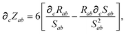
Noncovalent interactions are also particularly important in supramolecular chemistry, where non-bonded interactions such as dispersion, stabilize molecular assemblies. The large size of supramolecular host–guest complexes typically places them outside the reach of high-level quantum chemical methodologies and necessitates the use of DFT for geometry optimizations and energy computations. However, the large polarizable surfaces that interact in these systems requires a many-body treatment of dispersion to achieve a chemically accurate description of supramolecular binding energies.56,128 The C60 “buckyball catcher” host–guest complex (also referred to as C60@C60H28) in particular has received considerable attention as a benchmark supramolecular system in the hope that it is prototypical of dispersion-driven supramolecular systems, and it has been studied extensively both experimentally129–132 and theoretically.56,128,130,133–138 The C60 buckyball catcher (denoted as 4a by Grimme) is one of the most well studied members of the S12L test set of noncovalently bound supramolecular complexes.136
Much of the past computational work has focused on modeling the interaction energy of the C60 buckyball catcher and comparing these results to the experimental data on thermodynamic association constants that have been extracted from titration experiments.129–131 This complex is a challenging system for most dispersion correction methods since the three-body term contributes approximately 10% of the interaction energy.56,138 Motivated by this large contribution of beyond-pairwise dispersion, we optimized the C60@C60H28 complex with PBE+MBD, PBE+TS and PBE+D3 to see how significantly many-body effects impact the geometry. Containing 148 atoms, this system also represents a structure that would be too large to optimize with numerical MBD gradients or high-level wavefunction based methodologies. All theoretical calculations reported herein are for an isolated, i.e. gas-phase, host–guest complex in the classical equilibrium geometry at zero temperature.
The buckyball catcher host is made of a tetrabenzocyclooctatetraene (TBCOT) tether and two corannulene pincers (cf.Fig. 4 herein and Fig. S5 in the ESI†). The conformation of the catcher is determined by a competition between the attractive dispersion interactions between the corannulene pincers and the strain induced by deformation of the TBCOT tether.130 The two lowest energy “open” conformers of the catcher have the corannulene bowls in a convex–convex “catching” motif or in a convex–concave “waterwheel” motif; following the notation of ref. 129, 130 and 134 we term the “catching” motif a and the “waterwheel” motif b.
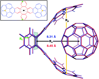 |
| | Fig. 4 Overlay between the geometry of the C60@C60H28 host–guest complex optimized with PBE+D3 (red) and PBE+MBD (blue). The distance, Rc, between the C60 centroid and the plane bisecting the tetrabenzocyclooctatetraene (TBCOT) tether (transparent green) is reduced from 8.45 Å with PBE+D3 to 8.31 Å with PBE+MBD. The green arrow shows that the Rt distance is measured between terminal carbon atoms on the TBCOT tether. The yellow arrow shows that the Rp distance is measured between the most separated carbon atoms of the central five-membered rings of both corannulene subunits. Inset: the 2D molecular structure of the C60H28 buckyball catcher host, with corannulene subunits shown in blue and the TBCOT tether shown in red. Atoms used to define the Rt and Rp distances are marked in green and yellow respectively. The black dot shows the centroid of the four atoms on the TBCOT tether used to define the Rc distance. | |
To compare the size of the cleft between the corannulene pincers when the buckyball catcher is optimized with various DFT+vdW methods, we report the distance between the most separated carbon atoms of the central five-membered rings of both corannulene subunits as a measure of the size of the cleft; we denote this distance as Rp (cf.Fig. 4). Closing of the cleft tends to be accompanied by outward deflection of the TBCOT tether, so we also measure the distance between terminal carbons on the tether; we denote this distance as Rt (cf.Fig. 4). Likewise, we measure the distance between the centroid of the C60 and the plane that bisects the TBCOT tether at the base of the buckyball catcher (cf.Fig. 4); we denote this distance as Rc. Interestingly, several of the functionals that have been used to study the buckyball catcher do not identify some conformers. Notably, TPSS-D3 is prone to drive conformer a to a closed variant that has Rc = 5.53 Å. With regard to the balance between dispersion and strain, conformer a results when the C60 is removed from the pincers and the host is allowed to relax. We will focus our discussion on the relaxed conformer a and the optimized complex, but we also provide optimized structures of conformer b in the ESI.†
Upon optimization with PBE+MBD we find that the corannulene pincers deflect outward, as seen by the increased Rp distance relative to the starting TPSS+D3/def2TZVP geometry from the S12L dataset.136 The Rp distance predicted by PBE+MBD is larger than other results from vdW-inclusive functionals (see Table 1), which is consistent with previous reports of three-body and higher order terms substantially decreasing the binding energy of the C60@C60H28 host–guest complex.56,138 However, this deflection is accompanied by a reduction of the buckyball-catcher distance Rc, which would suggest a tighter binding. Just as with the reduced cleft distances in the peptides and the inter-monomer distance in the benzene dimer, we find that the host–guest distance predicted by PBE+MBD (Rc = 8.31 Å) is smaller than that predicted by PBE+D3 (Rc = 8.45 Å) and PBE+TS (Rc = 8.36 Å). For comparison, we also optimized the complex with TPSS+D3/def2TZVP and found a buckyball-catcher distance of Rc = 8.39 Å, which is slightly larger than the Rc = 8.36 Å in the previously reported TPSS+D3/def2TZVP geometry in the S12L dataset.136 These results are reported in Table 1 together with a comparison to previous vdW-inclusive DFT results.
Table 1 Selected distances of DFT gas-phase optimized geometries of the C60@C60H28 host–guest complex and conformer a of the host alone. The TPSS functional does not identify conformer a, so these entries are left blank
| Method |
Complex |
Host a |
|
R
c (Å) |
R
p (Å) |
R
t (Å) |
R
p (Å) |
R
t (Å) |
|
Ref. 136.
Ref. 130.
Ref. 133.
|
| PBE+MBD |
8.312 |
12.992 |
6.303 |
13.263 |
6.394 |
| PBE+TS |
8.361 |
12.974 |
6.337 |
12.969 |
6.080 |
| PBE+D3 |
8.454 |
12.987 |
6.286 |
11.640 |
6.215 |
| TPSS+D3 |
8.392 |
12.748 |
6.288 |
— |
— |
| TPSS+D3a |
8.361 |
12.822 |
6.303 |
— |
— |
| B97-Db |
8.335 |
12.798 |
6.299 |
11.152 |
6.216 |
| M06-2Lc |
8.136 |
12.703 |
6.382 |
11.844 |
6.322 |
Perhaps the most unusual trend in Table 1 is the substantial opening of the cleft between the corannulene subunits, and the accompanying outward deflection of the TBCOT tether, when the isolated host is optimized with the PBE+MBD method. Comparing the Rp and Rt distances, we find an ordering of PBE+MBD > PBE+TS > PBE+D3. Mück-Lichtenfeld et al. previously found that the TBCOT tether is quite flexible, resulting in a shallow bending potential (see Fig. 2 of ref. 130) as the Rp distance is varied; using the B97-D functional and 6-31G* basis set, the energy of conformer b varies by only ∼1.3 kcal mol−1 as Rp is scanned from 10–14 Å.130 Comparing the energy of the buckyball catcher in the strained conformer that it adopts when hosting the buckyball to its energy when fully relaxed, we see that at the PBE+D3/def2TZVP level this strain energy is 1.02 kcal mol−1. This is consistent with the shallow bending potential found by Mück-Lichtenfeld et al. Given how flat this PES is, it is less surprising that the three vdW corrections considered give such different relaxed Rp distances for the isolated host.
The structure of the C60 buckyball does not vary significantly between different vdW-inclusive functionals. The PBE+MBD optimized structure of C60 has C–C bond lengths of 1.45192 (5) Å for bonds within five-membered rings (fusing pentagons and hexagons), and 1.39804 (3) Å for bonds fusing hexagonal rings; which compares favorably to the well known gas-phase electron diffraction results of 1.458 (6) Å and 1.401 (10) Å.139 This result is consistent with the short-range behavior of the range-separated PBE+MBD method, which essentially reduces to the bare PBE functional and does a good job of predicting C–C bond lengths.
In agreement with our results for the benzene dimer and polypeptides, we find that the PBE+MBD method yields structures that deviate from those provided by pairwise dispersion-inclusive functionals. The buckyball catcher complex is the most complex system studied herein in terms of its intricate geometry and non-local polarization behavior, so it would not be unreasonable to assume that PBE+MBD yields the most reliable results. However, because we do not have a benchmark comparison for the C60@C60H28 host–guest complex, we cannot truly evaluate the performance of any method, including PBE+MBD. Only future high-level wavefunction-based geometry optimizations of this gas-phase complex (or optimization of the full crystal structure for comparison to the experimental X-ray determined structure129) will settle any remaining questions regarding the geometry of the buckyball catcher complex.
In light of the lack of high-level wavefunction-based geometries to compare against, we conclude with a few comments about the computational efficiency of our method. Starting from the TPSS/def2TZVP structures from the S12L dataset, we were able to optimize the 148-atom complex with the PBE+MBD method in 68 BFGS steps in about 415 cpu hours, while the PBE+D3 optimization in ORCA took 34 BFGS steps in about 450 cpu hours.‡‡Given that ORCA uses redundant internal coordinates for geometry optimizations and the D3 correction is almost instantaneous to calculate, it is worth noting that the Cartesian coordinates optimization in QE with the much more costly MBD correction is roughly competitive.
4.4 The importance of ∂V
Our derivation of the nuclear MBD forces placed considerable emphasis on the importance of including the implicit coordinate dependence arising from the gradients of the Hirshfeld effective atomic volumes. To test how large of a contribution that the ∂V terms make to the MBD forces, we re-optimized the benzene dimers, this time setting ∂V = 0 explicitly. As shown in Fig. S2 in the ESI,† neglect of the Hirshfeld volume gradients does not have a large impact for this system, in which the dispersion forces are intermolecular; the mean RMSD becomes (16 ± 5) × 10−4 Å. This result is expected for this system because the Hirshfeld effective atomic volumes only change when neighboring atoms are moved. Not only is the benzene monomer fairly rigid, but the range separation employed in MBD means that the long-range tensor TLR, and correspondingly the MBD correction, is largely turned off within the benzene monomer (see Fig. S1 in the ESI†).
We expect a larger impact from Hirshfeld volume gradients for systems that are flexible and large enough for the damping function to have “turned on” the MBD correction. The case of polypeptide intramolecular dispersion interactions matches both of these criteria. As such, we computed the MBD forces on the final optimized geometries of all 76 peptide structures and analyzed the atom-by-atom difference in the forces computed with and without the Hirshfeld volume gradients.§§ As shown in Fig. 5, neglect of the Hirshfeld gradient causes a significant shift in the distribution of the MBD forces in the peptides, with a tendency to increase the forces from the lower peak from ∼2 × 10⁻⁴Eh/a.u. to ∼4 × 10⁻⁴Eh/a.u. Comparing the Cartesian components of the MBD forces across all atoms in all 76 structures we find that the deviations between MBD forces with and without the Hirshfeld volume gradients (F − F∂V=0) are approximately normally distributed with zero mean and a standard deviation of 2 × 10⁻⁴Eh/a.u. (see Fig. S3 in the ESI†). This leads to the norm of the force difference (||F − F∂V||) having a mean of (3.2 ± 1.7) × 10−4Eh/a.u., and a mean of the difference of norms of ||F|| − ||F∂V=0|| = (−5 ± 17) × 10−5Eh/a.u. Overall, neglect of the Hirshfeld gradients increases the nuclear forces and causes a long-tailed distribution of relative error that is peaked at ∼20%, but extends up to 400%. This large distribution of relative errors has the potential to significantly impact the predictive nature of ab initio molecular dynamics (AIMD) simulations run at the MBD level of theory that do not properly account for the analytical gradients of the Hirshfeld effective volumes. Given that this error would accumulate at every time step, combined with the fact that the MBD correction was found to be quite important in the geometry optimizations of the systems considered herein, we find that the neglect of the Hirshfeld effective volume gradients is an unacceptable approximation in AIMD. This finding is particularly true for large flexible molecular systems with significant intramolecular dispersion interactions since this error can cooperatively increase along any extended direction, i.e., along an alkane chain or polypeptide backbone.
 |
| | Fig. 5
Left: Gaussian kernel density estimate of the distributions of the norm ||·|| of MBD forces FMBD acting on each atom at the optimized geometries of 76 polypeptide structures. In blue, the MBD forces were computed with full Hirshfeld gradients (||F||); in yellow, the forces were computed with the Hirshfeld gradients ∂V set to zero (||F∂V=0||). Right: Gaussian kernel density estimate of the distribution of relative percentage error ||ΔF||/||F|| where ΔF ≡ F − F∂V=0 is the error incurred by setting the Hirshfeld gradients to zero. The distribution is peaked at approximately 20% but extends to values much greater than 100%. | |
5 Conclusions and future research
By developing analytical energy gradients of the range-separated MBD energy with respect to nuclear coordinates, we have enabled the first applications of MBD to full nuclear relaxations. By treating the gradients of the MBD energy correction analytically rather than numerically, we have reduced the number of self-consistent calculations that must be performed from 2 × (3N − 6) to 1, enabling treatment of much larger systems. Our derivation and implementation includes all implicit coordinate dependencies arising from the Hirshfeld charge density partitioning. In the gas-phase geometry optimizations considered herein, the implicit coordinate dependencies that arise from the Hirshfeld volume gradients resulted in significant changes to the MBD forces. The long-tailed distribution of relative error that we observed indicates that any future AIMD simulations employing MBD forces must include a full treatment of the Hirshfeld volume gradients, or the accumulation of error will negatively impact the simulation dynamics. Our careful treatment of these volume gradients paves the wave for future work to address how a self-consistent implementation of the MBD model will impact the electronic band structures of layered materials and intermolecular charge transfer couplings in molecular crystals. In this regard, a fully self-consistent treatment of MBD will also likely be required for energy conservation in AIMD simulations and the impact of self-consistency on the total DFT+MBD forces in general represents an interesting avenue for future research.
Consistent with previous findings that a many-body description of dispersion improves the binding energies of even small molecular dimers,52 we find that MBD forces significantly improve the structures of gas-phase molecular systems displaying both intermolecular and intramolecular dispersion interactions. In this regard, we find excellent agreement between the PBE+MBD optimized structures and the available reference data in our investigation of both the stationary points on the benzene dimer potential energy surface and the secondary structure of polypeptides. Notably, PBE+MBD consistently outperformed the pairwise PBE+D3(BJ), and effectively pairwise PBE+TS optimizations.
The first applications of MBD forces in this paper were restricted to gas-phase systems because computation of MBD gradients in the condensed phase, where periodic images of the unit cell must be considered, is substantially more challenging from a computational perspective. Converging the MBD energy in the condensed phase is demanding (from both the memory and computational points of view) due to a real-space supercell procedure that is required to support long-wavelength normal modes of CMBD. A forthcoming publication will describe the details of our implementation of the MBD forces for periodic systems, including careful treatment of parallelization and convergence criteria.81
Since MBD forces are very efficient to evaluate for gas-phase molecules, we are eager to explore the application of MBD to AIMD simulations. Many-body effects have previously been shown to be significant in modeling solvation and aggregation in solution79 and can lead to soft collective fluctuations that impact hydrophobic association140 and the entropic stabilization of hydrogen-bonded molecular crystals.62 We therefore anticipate that our many-body forces will be of interest for solvated simulations, such as estimates of the thermodynamic properties of metabolites141 and modeling novel electrolytes.142
Acknowledgements
We thank Alexandre Tkatchenko and Alberto Ambrosetti for useful discussions and for providing source code for the FHI-aims implementation of MBD. This research used resources of the Odyssey cluster supported by the FAS Division of Science, Research Computing Group at Harvard University, the National Energy Research Scientific Computing Center (NERSC), a DOE Office of Science User Facility supported by the Office of Science of the U.S. Department of Energy under Contract No. DE-AC02-05CH11231, the Texas Advanced Computing Center (TACC) at The University of Texas at Austin, the Extreme Science and Engineering Discovery Environment (XSEDE),143 which is supported by National Science Foundation Grant No. ACI-1053575, and the Argonne Leadership Computing Facility at Argonne National Laboratory, which is supported by the Office of Science of the U.S. Department of Energy under contract DE-AC02-06CH11357. M. A. B.-F. acknowledges support from the DOE Office of Science Graduate Fellowship Program, made possible in part by the American Recovery and Reinvestment Act of 2009, administered by ORISE-ORAU under Contract No. DE-AC05-06OR23100. T. M. acknowledges support from the National Science Foundation (NSF) Graduate Research Fellowship Program. R. A. D. and R. C. acknowledge support from the Scientific Discovery through Advanced Computing (SciDAC) program through the Department of Energy under Grant No. DE-SC0008626. A. A.-G. acknowledges support from the STC Center for Integrated Quantum Materials, NSF Grant No. DMR-1231319. All opinions expressed in this paper are the authors' and do not necessarily reflect the policies and views of DOE, ORAU, ORISE, or NSF.
References
-
A. J. Stone, The theory of intermolecular forces, Oxford University Press, Oxford, UK, 2nd edn, 2013 Search PubMed.
-
D. J. Wales, Energy landscapes, Cambridge University Press, Cambridge, UK, New York, 2003 Search PubMed.
-
V. A. Parsegian, van der Waals forces: a handbook for biologists, chemists, engineers, and physicists, Cambridge University Press, New York, 2006 Search PubMed.
-
J. N. Israelachvili, Intermolecular and surface forces, Academic Press, Burlington, MA, 3rd edn, 2011 Search PubMed.
- K. Rapcewicz and N. W. Ashcroft, Phys. Rev. B: Condens. Matter Mater. Phys., 1991, 44, 4032 CrossRef.
- J. F. Dobson and B. P. Dinte, Phys. Rev. Lett., 1996, 76, 1780 CrossRef CAS PubMed.
- Y. Andersson, D. C. Langreth and B. I. Lundqvist, Phys. Rev. Lett., 1996, 76, 102 CrossRef CAS PubMed.
- M. Elstner, P. Hobza, T. Frauenheim, S. Suhai and E. Kaxiras, J. Chem. Phys., 2001, 114, 5149 CrossRef CAS.
- X. Wu, M. C. Vargas, S. Nayak, V. Lotrich and G. Scoles, J. Chem. Phys., 2001, 115, 8748 CrossRef CAS.
- Q. Wu and W. Yang, J. Chem. Phys., 2002, 116, 515 CrossRef CAS.
- M. Dion, H. Rydberg, E. Schröder, D. C. Langreth and B. I. Lundqvist, Phys. Rev. Lett., 2004, 92, 246401 CrossRef CAS PubMed.
- O. A. von Lilienfeld, I. Tavernelli, U. Rothlisberger and D. Sebastiani, Phys. Rev. Lett., 2004, 93, 153004 CrossRef PubMed.
- S. Grimme, J. Comput. Chem., 2004, 25, 1463 CrossRef CAS PubMed.
- A. J. Misquitta, R. Podeszwa, B. Jeziorski and K. Szalewicz, J. Chem. Phys., 2005, 123, 214103 CrossRef PubMed.
- A. D. Becke and E. R. Johnson, J. Chem. Phys., 2005, 122, 154104 CrossRef PubMed.
- A. D. Becke and E. R. Johnson, J. Chem. Phys., 2005, 123, 154101 CrossRef PubMed.
- E. R. Johnson and A. D. Becke, J. Chem. Phys., 2005, 123, 024101 CrossRef PubMed.
- S. Grimme, J. Comput. Chem., 2006, 27, 1787 CrossRef CAS PubMed.
- A. D. Becke and E. R. Johnson, J. Chem. Phys., 2006, 124, 014104 CrossRef PubMed.
- Y. Zhao and D. G. Truhlar, J. Chem. Phys., 2006, 125, 194101 CrossRef PubMed.
- A. D. Becke and E. R. Johnson, J. Chem. Phys., 2007, 127, 124108 CrossRef PubMed.
- A. D. Becke and E. R. Johnson, J. Chem. Phys., 2007, 127, 154108 CrossRef PubMed.
- P. Jurečka, J. Černý, P. Hobza and D. R. Salahub, J. Comput. Chem., 2007, 28, 555 CrossRef PubMed.
- P. L. Silvestrelli, Phys. Rev. Lett., 2008, 100, 053002 CrossRef PubMed.
- Y. Y. Sun, Y.-H. Kim, K. Lee and S. B. Zhang, J. Chem. Phys., 2008, 129, 154102 CrossRef CAS PubMed.
- J.-D. Chai and M. Head-Gordon, Phys. Chem. Chem. Phys., 2008, 10, 6615 RSC.
- G. A. DiLabio, Chem. Phys. Lett., 2008, 455, 348 CrossRef CAS.
- I. D. Mackie and G. A. DiLabio, J. Phys. Chem. A, 2008, 112, 10968 CrossRef CAS PubMed.
- A. Tkatchenko and M. Scheffler, Phys. Rev. Lett., 2009, 102, 073005 CrossRef PubMed.
- G. Román-Pérez and J. M. Soler, Phys. Rev. Lett., 2009, 103, 096102 CrossRef PubMed.
- O. A. Vydrov and T. van Voorhis, Phys. Rev. Lett., 2009, 103, 063004 CrossRef PubMed.
- E. R. Johnson and G. A. DiLabio, J. Phys. Chem. C, 2009, 113, 5681 CAS.
- T. Sato and H. Nakai, J. Chem. Phys., 2009, 131, 224104 CrossRef PubMed.
- T. Sato and H. Nakai, J. Chem. Phys., 2010, 133, 194101 CrossRef PubMed.
- S. Grimme, J. Antony, S. Ehrlich and H. Krieg, J. Chem. Phys., 2010, 132, 154104 CrossRef PubMed.
- A. Tkatchenko, L. Romaner, O. T. Hofmann, E. Zojer, C. Ambrosch-Draxl and M. Scheffler, MRS Bull., 2010, 35, 435 CrossRef CAS.
- V. R. Cooper, L. Kong and D. C. Langreth, Phys. Procedia, 2010, 3, 1417 CrossRef CAS.
- K. E. Riley, M. Pitoňák, P. Jurečka and P. Hobza, Chem. Rev., 2010, 110, 5023 CrossRef CAS PubMed.
- F. O. Kannemann and A. D. Becke, J. Chem. Theory Comput., 2010, 6, 1081 CrossRef CAS.
- O. A. Vydrov and T. V. Voorhis, J. Chem. Phys., 2010, 133, 244103 CrossRef PubMed.
- K. Lee, É. D. Murray, L. Kong, B. I. Lundqvist and D. C. Langreth, Phys. Rev. B: Condens. Matter Mater. Phys., 2010, 82, 081101(R) CrossRef.
- S. Grimme, Wiley Interdiscip. Rev.: Comput. Mol. Sci., 2011, 1, 211 CrossRef CAS.
- S. N. Steinmann and C. Corminboeuf, J. Chem. Theory Comput., 2011, 7, 3567 CrossRef CAS PubMed.
- N. Marom, A. Tkatchenko, M. Rossi, V. V. Gobre, O. Hod, M. Scheffler and L. Kronik, J. Chem. Theory Comput., 2011, 7, 3944 CrossRef CAS PubMed.
- S. Grimme, S. Ehrlich and L. Goerigk, J. Comput. Chem., 2011, 32, 1456 CrossRef CAS PubMed.
- A. Tkatchenko, R. A. DiStasio Jr, R. Car and M. Scheffler, Phys. Rev. Lett., 2012, 108, 236402 CrossRef PubMed.
- R. A. DiStasio Jr, O. A. von Lilienfeld and A. Tkatchenko, Proc. Natl. Acad. Sci. U. S. A., 2012, 109, 14791 CrossRef PubMed.
- E. Torres and G. A. DiLabio, J. Phys. Chem. Lett., 2012, 3, 1738 CrossRef CAS PubMed.
- A. Tkatchenko, A. Ambrosetti and R. A. DiStasio Jr, J. Chem. Phys., 2013, 138, 074106 CrossRef PubMed.
- R. Sabatini, T. Gorni and S. de Gironcoli, Phys. Rev. B: Condens. Matter Mater. Phys., 2013, 87, 041108(R) CrossRef.
- P. L. Silvestrelli, J. Chem. Phys., 2013, 139, 054106 CrossRef PubMed.
- R. A. DiStasio Jr, V. V. Gobre and A. Tkatchenko, J. Phys.: Condens. Matter, 2014, 26, 213202 CrossRef PubMed.
- A. Ambrosetti, A. M. Reilly, R. A. DiStasio Jr and A. Tkatchenko, J. Chem. Phys., 2014, 140, 18A508 CrossRef PubMed.
- A. D. Becke, J. Chem. Phys., 2014, 140, 18A301 CrossRef PubMed.
- J. Klimeš and A. Michaelides, J. Chem. Phys., 2012, 137, 120901 CrossRef PubMed.
- A. Ambrosetti, D. Alfé, R. A. DiStasio Jr and A. Tkatchenko, J. Phys. Chem. Lett., 2014, 5, 849 CrossRef CAS PubMed.
- A. Tkatchenko, M. Rossi, V. Blum, J. Ireta and M. Scheffler, Phys. Rev. Lett., 2011, 106, 118102 CrossRef PubMed.
- A. Otero de la Roza and E. R. Johnson, J. Chem. Phys., 2012, 137, 054103 CrossRef CAS PubMed.
- A. M. Reilly and A. Tkatchenko, J. Chem. Phys., 2013, 139, 024705 CrossRef PubMed.
- A. M. Reilly and A. Tkatchenko, J. Phys. Chem. Lett., 2013, 4, 1028 CrossRef CAS PubMed.
- N. Marom, R. A. DiStasio Jr, V. Atalla, S. Levchenko, A. M. Reilly, J. R. Chelikowsky, L. Leiserowitz and A. Tkatchenko, Angew. Chem., Int. Ed., 2013, 52, 6629 CrossRef CAS PubMed.
- A. M. Reilly and A. Tkatchenko, Phys. Rev. Lett., 2014, 113, 055701 CrossRef PubMed.
- L. Kronik and A. Tkatchenko, Acc. Chem. Res., 2014, 47, 3208 CrossRef CAS PubMed.
- Y. V. Shtogun and L. M. Woods, J. Phys. Chem. Lett., 2010, 1, 1356 CrossRef CAS.
- T. Björkman, A. Gulans, A. Krasheninnikov and R. M. Nieminen, Phys. Rev. Lett., 2012, 108, 235502 CrossRef PubMed.
- B. M. Axilrod and E. Teller, J. Chem. Phys., 1943, 11, 299 CrossRef CAS.
- Y. Muto, Proc. Phys.-Math. Soc. Jpn., 1943, 17, 629 CAS.
- J. F. Dobson and T. Gould, J. Phys.: Condens. Matter, 2012, 24, 073201 CrossRef PubMed.
- A. M. Reilly and A. Tkatchenko, Chem. Sci., 2015, 6, 3289 RSC.
- C. Wagner, N. Fournier, V. G. Ruiz, C. Li, K. Müllen, M. Rohlfing, A. Tkatchenko, R. Temirov and F. S. Tautz, Nat. Commun., 2014, 5, 5568 CrossRef CAS PubMed.
- F. L. Hirshfeld, Theor. Chim. Acta, 1977, 44, 129 CrossRef CAS.
- R. F. Nalewajski and R. G. Parr, Proc. Natl. Acad. Sci. U. S. A., 2000, 97, 8879 CrossRef CAS.
- K. T. Tang and M. Karplus, Phys. Rev., 1968, 171, 70 CrossRef CAS.
- T. Brinck, J. S. Murray and P. Politzer, J. Chem. Phys., 1993, 98, 4305 CrossRef CAS.
- P. Bultinck, C. van Alsenoy, P. W. Ayers and R. Carbó-Dorca, J. Chem. Phys., 2007, 126, 144111 CrossRef PubMed.
- N. Ferri, R. A. DiStasio Jr, A. Ambrosetti, R. Car and A. Tkatchenko, Phys. Rev. Lett., 2015, 114, 176802 CrossRef PubMed.
- B. Thole, Chem. Phys., 1981, 59, 341 CrossRef CAS.
- H. B. G. Casimir and D. Polder, Phys. Rev., 1948, 73, 360 CrossRef CAS.
- A. G. Donchev, J. Chem. Phys., 2006, 125, 074713 CrossRef CAS PubMed.
- P. Giannozzi, S. Baroni, N. Bonini, M. Calandra, R. Car, C. Cavazzoni, D. Ceresoli, G. L. Chiarotti, M. Cococcioni, I. Dabo, A. Dal Corso, S. de Gironcoli, S. Fabris, G. Fratesi, R. Gebauer, U. Gerstmann, C. Gougoussis, A. Kokalj, M. Lazzeri, L. Martin-Samos, N. Marzari, F. Mauri, R. Mazzarello, S. Paolini, A. Pasquarello, L. Paulatto, C. Sbraccia, S. Scandolo, G. Sclauzero, A. P. Seitsonen, A. Smogunov, P. Umari and R. M. Wentzcovitch, J. Phys.: Condens. Matter, 2009, 21, 395502 CrossRef PubMed.
-
T. Markovich, M. A. Blood-Forsythe, R. A. DiStasio Jr and A. Aspuru-Guzik, unpublished.
-
T. Helgaker, P. Jørgensen and J. Olsen, Molecular electronic-structure theory, Wiley, Chichester, New York, 2000 Search PubMed.
- A. Bondi, J. Phys. Chem., 1964, 68, 441 CrossRef CAS.
- P. Bendt and A. Zunger, Phys. Rev. Lett., 1983, 50, 1684 CrossRef CAS.
- G. Srivastava and D. Weaire, Adv. Phys., 1987, 36, 463 CrossRef CAS.
-
D. Marx and J. Hutter, Ab Initio Molecular Dynamics: Basic Theory and Advanced Methods, Cambridge University Press, Cambridge, UK, New York, 2009 Search PubMed.
- R. B. Nelson, AIAA J., 1976, 14, 1201 CrossRef.
- J. P. Perdew, K. Burke and M. Ernzerhof, Phys. Rev. Lett., 1996, 77, 3865 CrossRef CAS PubMed.
- J. P. Perdew, K. Burke and M. Ernzerhof, Phys. Rev. Lett., 1997, 78, 1396 CrossRef CAS.
- D. R. Hamann, M. Schlüter and C. Chiang, Phys. Rev. Lett., 1979, 43, 1494 CrossRef CAS.
- G. B. Bachelet, D. R. Hamann and M. Schlüter, Phys. Rev. B: Condens. Matter Mater. Phys., 1982, 26, 4199 CrossRef CAS.
- D. Vanderbilt, Phys. Rev. B: Condens. Matter Mater. Phys., 1985, 32, 8412 CrossRef CAS.
- F. Neese, Wiley Interdiscip. Rev.: Comput. Mol. Sci., 2012, 2, 73 CrossRef CAS.
- V. Blum, R. Gehrke, F. Hanke, P. Havu, V. Havu, X. Ren, K. Reuter and M. Scheffler, Comput. Phys. Commun., 2009, 180, 2175 CrossRef CAS.
- A. Tkatchenko, MBD@rsSCS, http://th.fhi-berlin.mpg.de/%7Etkatchen/MBD.
- P. Hobza, H. L. Selzle and E. W. Schlag, J. Chem. Phys., 1990, 93, 5893 CrossRef CAS.
- E. Arunan and H. S. Gutowsky, J. Chem. Phys., 1993, 98, 4294 CrossRef CAS.
- P. Hobza, H. L. Selzle and E. W. Schlag, J. Phys. Chem., 1993, 97, 3937 CrossRef CAS.
- P. Hobza, H. L. Selzle and E. W. Schlag, J. Am. Chem. Soc., 1994, 116, 3500 CrossRef CAS.
- R. L. Jaffe and G. D. Smith, J. Chem. Phys., 1996, 105, 2780 CrossRef CAS.
- P. Hobza, H. L. Selzle and E. W. Schlag, J. Phys. Chem., 1996, 100, 18790 CrossRef CAS.
- J. Gauss and J. F. Stanton, J. Phys. Chem. A, 2000, 104, 2865 CrossRef CAS.
- S. Tsuzuki, K. Honda, T. Uchimaru, M. Mikami and K. Tanabe, J. Am. Chem. Soc., 2002, 124, 104 CrossRef CAS PubMed.
- M. O. Sinnokrot, E. F. Valeev and C. D. Sherrill, J. Am. Chem. Soc., 2002, 124, 10887 CrossRef CAS PubMed.
- M. O. Sinnokrot and C. D. Sherrill, J. Phys. Chem. A, 2004, 108, 10200 CrossRef CAS.
- T. P. Tauer and C. D. Sherrill, J. Phys. Chem. A, 2005, 109, 10475 CrossRef CAS PubMed.
- R. Podeszwa, R. Bukowski and K. Szalewicz, J. Phys. Chem. A, 2006, 110, 10345 CrossRef CAS PubMed.
- J. Grant Hill, J. A. Platts and H.-J. Werner, Phys. Chem. Chem. Phys., 2006, 8, 4072 RSC.
- R. A. DiStasio Jr, G. von Helden, R. P. Steele and M. Head-Gordon, Chem. Phys. Lett., 2007, 437, 277 CrossRef.
- T. Janowski and P. Pulay, Chem. Phys. Lett., 2007, 447, 27 CrossRef CAS.
- E. C. Lee, D. Kim, P. Jurečka, P. Tarakeshwar, P. Hobza and K. S. Kim, J. Phys. Chem. A, 2007, 111, 3446 CrossRef CAS PubMed.
- B. Fernández, T. B. Pedersen, A. Sánchez
de Merás and H. Koch, Chem. Phys. Lett., 2007, 441, 332 CrossRef.
- O. Bludský, M. Rubeš, P. Soldán and P. Nachtigall, J. Chem. Phys., 2008, 128, 114102 CrossRef PubMed.
- M. Pavone, N. Rega and V. Barone, Chem. Phys. Lett., 2008, 452, 333 CrossRef CAS.
- M. Pitoňak, P. Neogrády, J. Řezáč, P. Jurečka, M. Urban and P. Hobza, J. Chem. Theory Comput., 2008, 4, 1829 CrossRef.
- C. D. Sherrill, T. Takatani and E. G. Hohenstein, J. Phys. Chem. A, 2009, 113, 10146 CrossRef CAS PubMed.
- J. Gräfenstein and D. Cremer, J. Chem. Phys., 2009, 130, 124105 CrossRef PubMed.
- O. A. von Lilienfeld and A. Tkatchenko, J. Chem. Phys., 2010, 132, 234109 CrossRef PubMed.
- H. Valdes, K. Pluháčková, M. Pitonak, J. Řezáč and P. Hobza, Phys. Chem. Chem. Phys., 2008, 10, 2747 RSC.
- C. Møller and M. S. Plesset, Phys. Rev., 1934, 46, 618 CrossRef.
- E. Baerends, D. Ellis and P. Ros, Chem. Phys., 1973, 2, 41 CrossRef CAS.
- B. I. Dunlap, J. W. D. Connolly and J. R. Sabin, J. Chem. Phys., 1979, 71, 3396 CrossRef CAS.
- F. Weigend, M. Häser, H. Patzelt and R. Ahlrichs, Chem. Phys. Lett., 1998, 294, 143 CrossRef CAS.
- T. H. Dunning, J. Chem. Phys., 1989, 90, 1007 CrossRef CAS.
-
J. W. Tukey, Exploratory data analysis, Addison-Wesley Pub. Co, Reading, MA, 1977 Search PubMed.
- A. Tkatchenko, R. A. DiStasio Jr, M. Head-Gordon and M. Scheffler, J. Chem. Phys., 2009, 131, 094106 CrossRef PubMed.
- S. Grimme, J. G. Brandenburg, C. Bannwarth and A. Hansen, J. Chem. Phys., 2015, 143, 054107 CrossRef PubMed.
- A. Tkatchenko, D. Alfé and K. S. Kim, J. Chem. Theory Comput., 2012, 8, 4317 CrossRef CAS PubMed.
- A. Sygula, F. R. Fronczek, R. Sygula, P. W. Rabideau and M. M. Olmstead, J. Am. Chem. Soc., 2007, 129, 3842 CrossRef CAS PubMed.
- C. Mück-Lichtenfeld, S. Grimme, L. Kobryn and A. Sygula, Phys. Chem. Chem. Phys., 2010, 12, 7091 RSC.
- V. H. Le, M. Yanney, M. McGuire, A. Sygula and E. A. Lewis, J. Phys. Chem. B, 2014, 118, 11956 CrossRef CAS PubMed.
- A. V. Zabula, Y. V. Sevryugina, S. N. Spisak, L. Kobryn, R. Sygula, A. Sygula and M. A. Petrukhina, Chem. Commun., 2014, 50, 2657 RSC.
- Y. Zhao and D. G. Truhlar, Phys. Chem. Chem. Phys., 2008, 10, 2813 RSC.
- M. P. Waller, H. Kruse, C. Mück-Lichtenfeld and S. Grimme, Chem. Soc. Rev., 2012, 41, 3119 RSC.
- R. Podeszwa, W. Cencek and K. Szalewicz, J. Chem. Theory Comput., 2012, 8, 1963 CrossRef CAS PubMed.
- S. Grimme, Chem.–Eur. J., 2012, 18, 9955 CrossRef CAS PubMed.
- P. A. Denis, RSC Adv., 2013, 3, 25296 RSC.
- T. Risthaus and S. Grimme, J. Chem. Theory Comput., 2013, 9, 1580 CrossRef CAS PubMed.
- K. Hedberg, L. Hedberg, D. S. Bethune, C. Brown, H. Dorn, R. D. Johnson and M. de Vries, Science, 1991, 254, 410 CAS.
- A. Godec, J. C. Smith and F. Merzel, Phys. Rev. Lett., 2013, 111, 127801 CrossRef PubMed.
- A. Jinich, D. Rappoport, I. Dunn, B. Sanchez-Lengeling, R. Olivares-Amaya, E. Noor, A. B. Even and A. Aspuru-Guzik, Sci. Rep., 2014, 4, 7022 CrossRef CAS PubMed.
- S. Er, C. Suh, M. P. Marshak and A. Aspuru-Guzik, Chem. Sci., 2015, 6, 885 RSC.
- J. Towns, T. Cockerill, M. Dahan, I. Foster, K. Gaither, A. Grimshaw, V. Hazlewood, S. Lathrop, D. Lifka, G. D. Peterson, R. Roskies, J. R. Scott and N. Wilkens-Diehr, Comput. Sci. Eng., 2014, 16, 62 CrossRef.
Footnotes |
| † Electronic supplementary information (ESI) available: The ESI contains additional derivation details, a comprehensive symbol glossary, and Cartesian coordinates for all structures considered in this work. See DOI: 10.1039/c5sc03234b |
| ‡ These authors contributed equally to this work. |
| § Although there are numerous schemes for partitioning the electron density, the Hirshfeld prescription71 has been shown to result in atomic partitions that most closely resemble the densities of the corresponding free (isolated) atoms (by minimizing the Kullback–Leibler entropy deficiency of information theory).72 |
| ¶ The dipole polarizability tensor αa for a given atom or QHO is formed by populating the diagonal elements (αxx, αyy, αzz) with the isotropic dipole polarizability in eqn (7). |
|| At this point, it is very important to note a difference in the notation relative to ref. 49 and 52: our matrix  is equivalent to their is equivalent to their  or B, which was keeping with Thole's original notation77 for the relay matrix. or B, which was keeping with Thole's original notation77 for the relay matrix. |
| ** Since each QHO is assigned a unit charge (e = 1), the dipole moment μ is thereby equivalent to the displacement vector ξ. |
| †† It is very important to note that in this work we have only computed the Hellmann–Feynman derivative of the total DFT+MBD energy. Specifically, when the MBD energy is computed non-self-consistently (i.e. as an a posteriori correction), there is an additional force component that results from the gradient of the molecular orbital coefficients (i.e., the non-self-consistency correction).84–86 This term can be treated by directly computing the “response” of the density by solving the coupled-perturbed-Kohn–Sham equations. Alternatively, this term exactly vanishes if MBD is computed self-consistently, which is our recommended approach. |
| ‡‡ The PBE+MBD optimization was run in about 2.75 hours on 170 Intel Xeon E5-2680 processors while the PBE+D3 optimization was run in about 14 hours on 32 AMD Opteron 6376 Abu Dhabi processors. |
| §§ Since the TS method is also based on Hirshfeld partitioning, the Hirshfeld volume gradients are also expected to be significant when computing the TS nuclear forces. A similar analysis of the TS forces on these peptide structures is provided in the ESI.† |
|
| This journal is © The Royal Society of Chemistry 2016 |
Click here to see how this site uses Cookies. View our privacy policy here. 
 Open Access Article
 This Open Access Article is licensed under a Creative Commons Attribution-Non Commercial 3.0 Unported Licence
 a,
Thomas
Markovich‡
a,
Thomas
Markovich‡
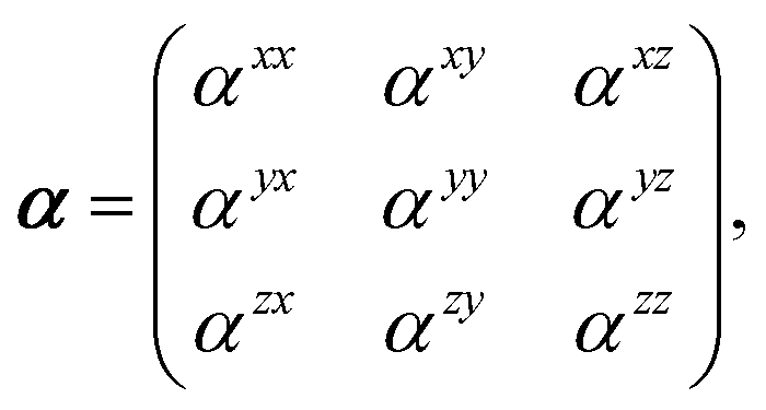
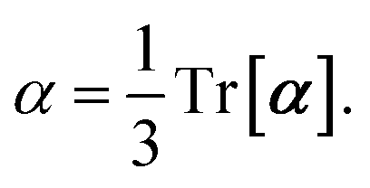
 . For brevity we will refer to the MBD@rsSCS model (which has also been denoted as MBD* elsewhere) as simply MBD throughout the manuscript.
 . The internuclear vector is denoted
  , such that the internuclear distance is given by Rab = ||Rab||. It follows that the ith Cartesian component of this internuclear vector is Riab. Finally, the effective vdW radius of an atom a is indicated by
  .
. will arise both explicitly through the presence of internuclear distance terms, Rab, and implicitly through the presence of effective atomic volume terms,
  , obtained via the Hirshfeld partitioning71 of ρ(r) (see Section 2.2.1). As such, these distinct types of dependence on the nuclear positions will be clearly delineated throughout the review of the MBD model and the derivation of the corresponding MBD nuclear forces below. For notational convenience, we will often use ∂c rather than
 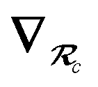 to indicate a derivative with respect to the nuclear position of atom c.
 (see Section 2.2.2). The MBD model Hamiltonian is then constructed based on these screened frequency-dependent dipole polarizabilities. Diagonalization of this Hamiltonian couples this collection of QHOs within the dipole approximation, yielding a set of interacting QHO eigenmodes with corresponding eigenfrequencies {λ}. The difference between the zero-point energy of these interacting QHO eigenmodes and that of the input non-interacting modes
  , is then used to compute the long-range correlation energy at the MBD level of theory (see Section 2.2.3), i.e.,
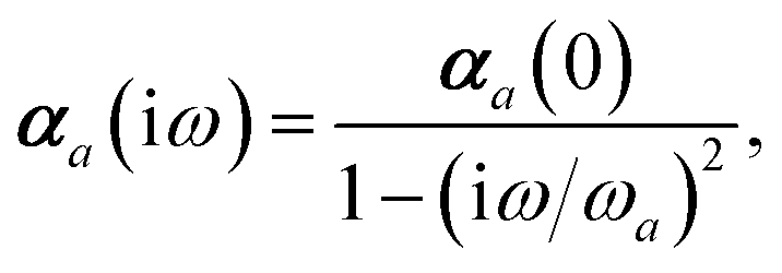

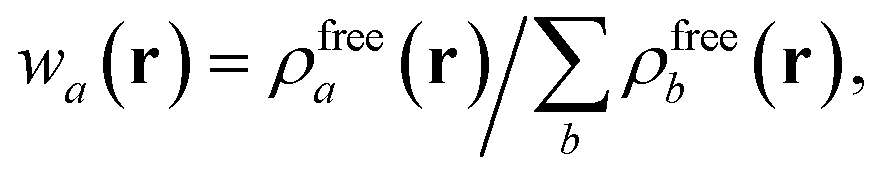
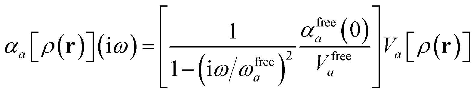
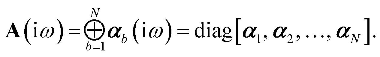
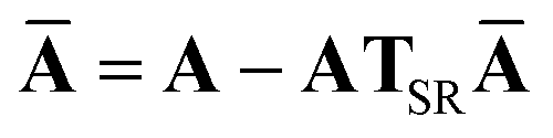
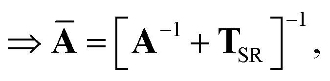
 is the (dense) screened non-local polarizability matrix, sometimes called the relay matrix.||
 yields the screened and anisotropic atomic polarizability tensors (the corresponding molecular polarizability is obtained by total internal contraction), i.e.,
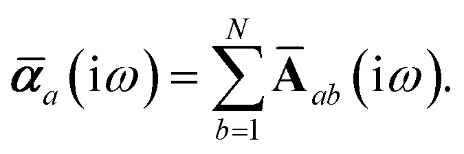
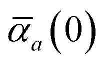 , that appear in the MBD Hamiltonian in eqn (17) and Section 2.2.3 below are then calculated from
  via
via
 to
to  . However, the relationship between
  and
and  , given in eqn (15), is one that is derived from the Padé approximant for the bare polarizability α(
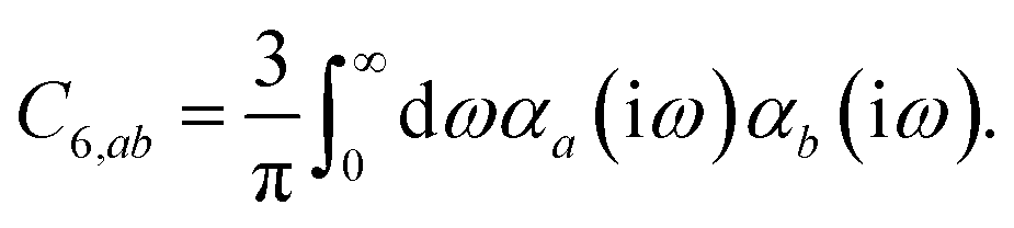
 , can be determined by a Gauss–Legendre quadrature estimate of the integral in eqn (14). The screened QHO characteristic excitation frequency,
  , is then calculated as
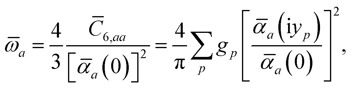
 , and acquire instantaneous dipole moments, da = qaxa, that are proportional to the displacement, xa, from the equilibrium position and charge, qa, on each oscillator. This Hamiltonian defines the so-called coupled fluctuating dipole model (CFDM),79 and is given by:
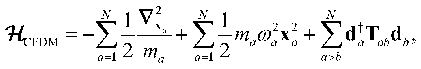
 (as defined in Section 2.2.4 and eqn (37) below), and the fluctuating point dipoles are replaced with the Gaussian charge densities of QHOs, with effective masses
 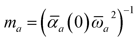 obtained from their respective static polarizabilities and excitation frequencies. The corresponding range-separated MBD model Hamiltonian is therefore:53
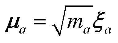 is the mass-weighted dipole moment of QHO a that has been displaced by ξa from its equilibrium position.** The first two terms in eqn (17) represent the kinetic and potential energy of the individual QHOs, respectively, and the third term is the two-body coupling due to the long-range dipole–dipole interaction tensor,
  , defined below in eqn (37).

 correspond to the modes of the non-interacting reference system of screened oscillators. The MBD correlation energy is then evaluated viaeqn (3) as the zero-point energetic difference between the interacting and non-interacting modes.
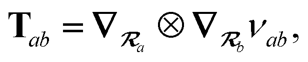

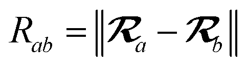 ,
,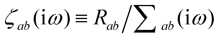
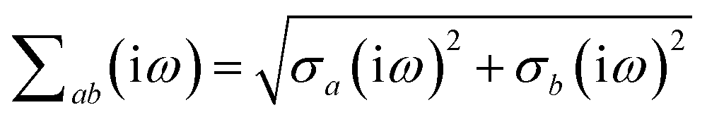
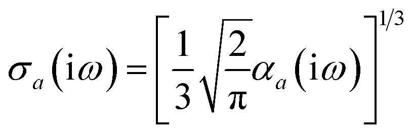

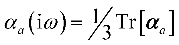 is the “isotropized” bare dipole polarizability and eqn (8) was used to make the effective volume dependence more explicit.
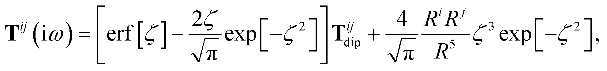

 :
: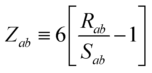
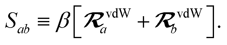
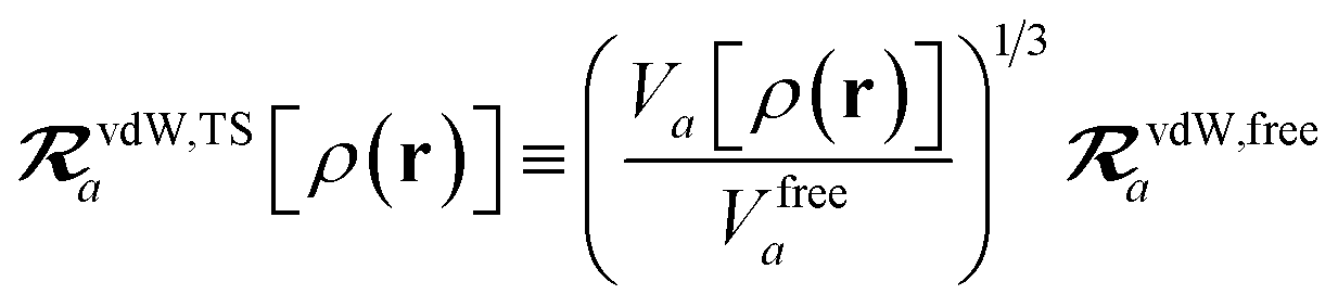
 is the free-atom vdW radius defined in ref. 29 using an electron density contour, not the Bondi83 radius that corresponds to the “atom-in-a-molecule” analog of this quantity. To indicate that the TS-level effective vdW radii are being used, the argument of the damping function for the short-range interaction tensor, used in eqn (10) and (11), will be denoted with ZTS (cf.eqn (29), (30) and (34)):
 takes the place of V/Vfree thereby still exploiting the proportionality between polarizability and volume.52,74 To indicate that the screened effective vdW radii are being used, the argument of the damping function for the long-range interaction tensor will be denoted with
  (cf.eqn (29), (30) and (36)):
 is why we use an overline on TLR above, and in eqn (17) and (18).
 of an arbitrary atom c.††
 and implicit dependence through
  (as moving a neighboring atom c will slightly alter the effective volume assigned to atom a). Future work will address the effects of the MBD contribution to the exchange–correlation potential when applied self-consistently, which will ultimately impact ρ(r). Our current work neglects these effects, and computes MBD as an a posteriori correction to DFT, i.e., non-self-consistently.
 in the relevant quantities above, the derivation proceeds largely by brute force application of the chain and product rules. The derivative of the MBD correlation energy given in eqn (3) is governed by:
 , as well as the eigenvalues, λp, of the CMBD matrix. Since CMBD is real and symmetric, it has 3N orthogonal eigenvectors. We therefore do not concern ourselves here with repeated eigenvalues (see the ESI† for a more detailed discussion) and take derivatives of λp as:87
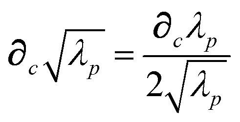
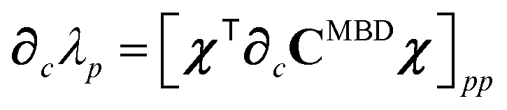
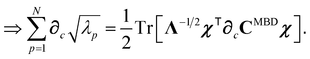
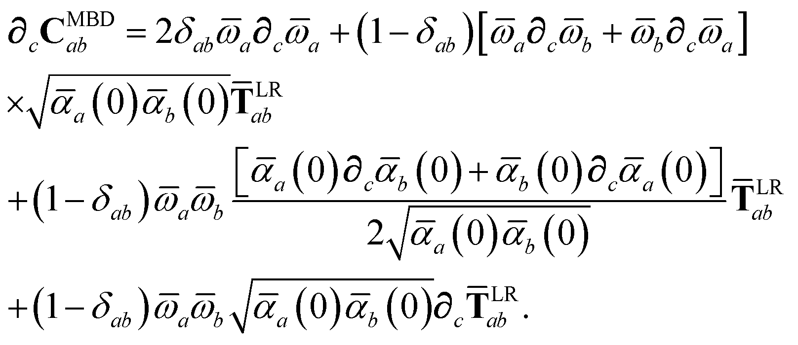
 ,
,  , and
, and  . From eqn (15), we find that the derivative of the screened excitation frequency,
  , requires us to evaluate derivatives of
  (with
(with 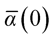 as a specific case) as follows:
 , eqn (13), is calculated from the “isotropized” partial contraction of
  (with the frequency dependence suppressed):
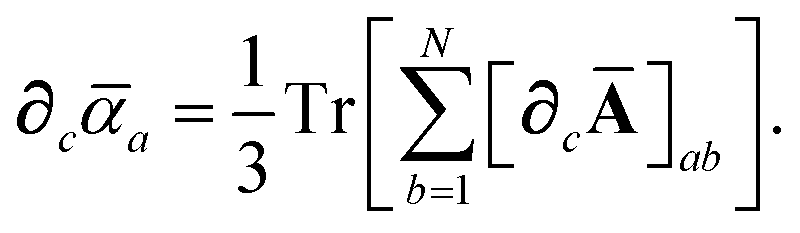
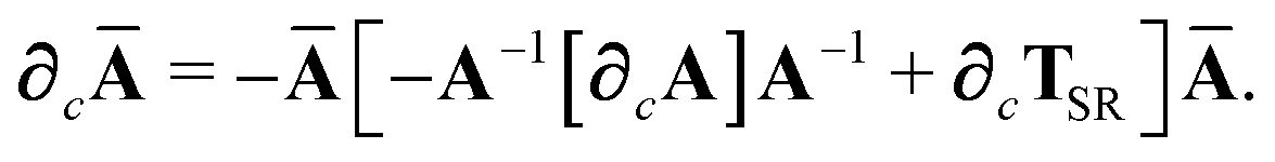

 , eqn (37), are fairly complicated, so it will help to consider first the damping function, f, in isolation. Here,
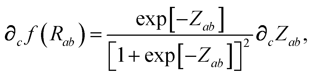
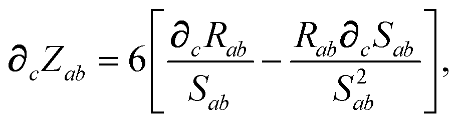
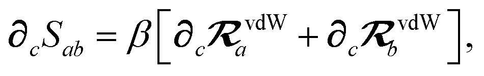
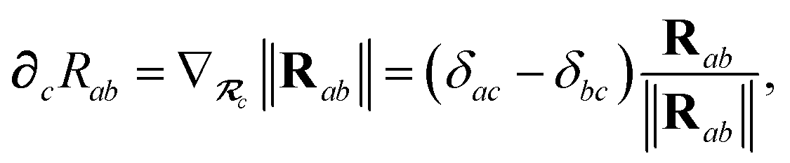

 , eqn (37), we require the derivative of the screened effective vdW radii, eqn (36):
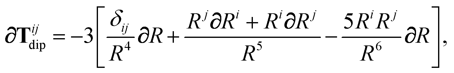

 as:
as: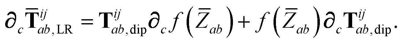

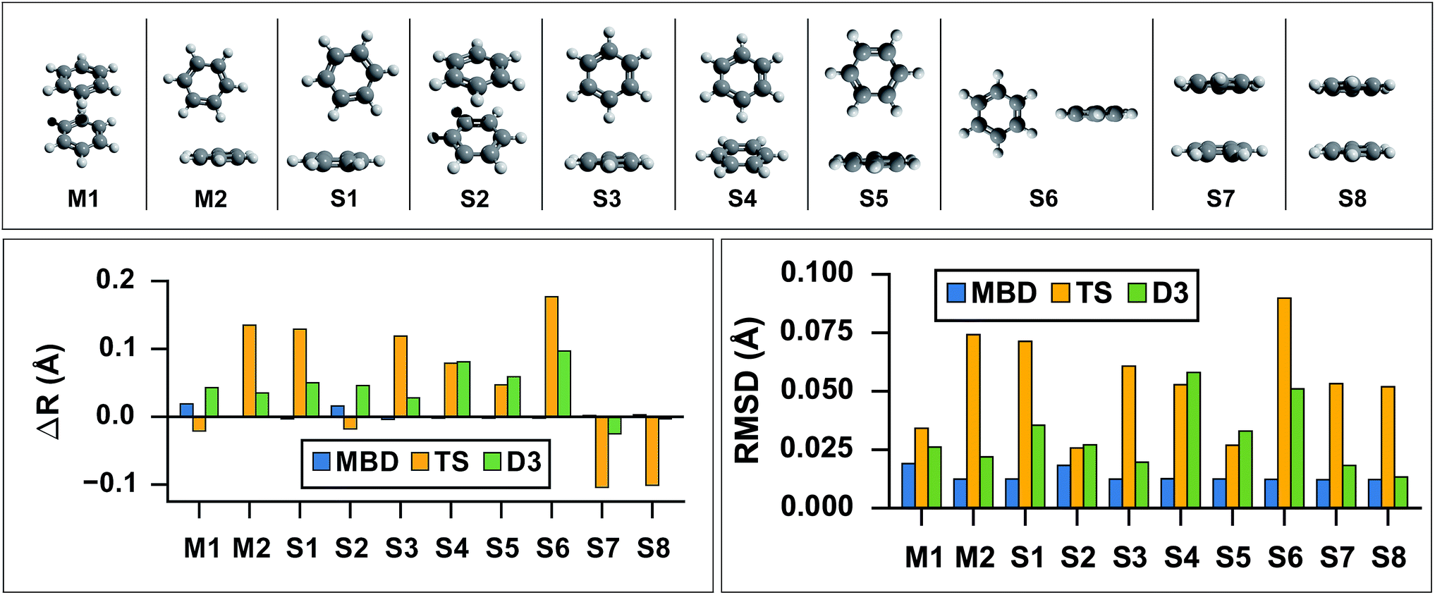
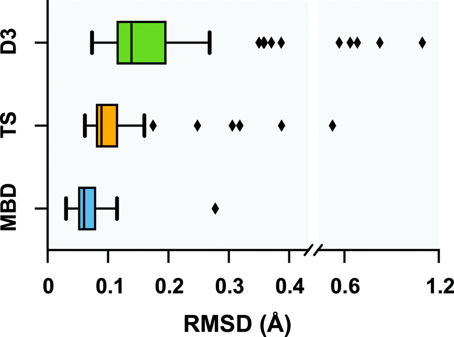
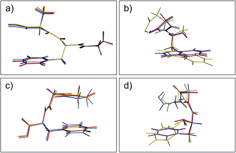

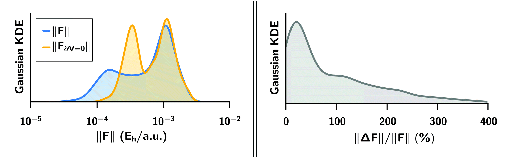
 is equivalent to their
  or B, which was keeping with Thole's original notation77 for the relay matrix.