
 Open Access Article
 This Open Access Article is licensed under a
 Creative Commons Attribution 3.0 Unported Licence
Application of vibrational spectroscopy techniques to non-destructively monitor plant health and development†
Holly J.
Butler
ab,
Martin R.
McAinsh
*c,
Steven
Adams
d and
Francis L.
Martin
*a
aCentre for Biophotonics, Lancaster University, Lancaster LA1 4YQ, UK. E-mail: f.martin@lancaster.ac.uk; Tel: +44 (0)1524 510206
bCentre for Global Eco-Innovation, Lancaster University, Lancaster LA1 4YQ, UK
cLancaster Environment Centre, Lancaster University, Lancaster LA1 4YQ, UK. E-mail: m.mcainsh@lancaster.ac.uk; Tel: +44 (0)1524 510553
dPlant Impact Plc, Rothamsted, West Common, Harpenden, Hertfordshire AL5 2JQ, UK
First published on 2nd April 2015
Abstract
Vibrational spectroscopy is a powerful analytical tool that is yet to be fully developed in plant science. Previously, such tools have been primarily applied to fixed or in vitro biological materials, which do not effectively encapsulate real-time physiological conditions of whole organisms. Coupled with multivariate analysis, this study examines the potential application of ATR-FTIR or Raman spectroscopy to determine spectral alterations indicative of healthy plant growth in leaf samples of Solanum lycopersicum. This was achieved in the absence of destructive effects on leaf tissues locally or on plant health systemically; additionally, autofluorescence was not a confounder. Feature extraction techniques including PCA-LDA were employed to examine variance within spectral datasets. In vivo measurements are able to successfully characterise key constituents of the leaf cuticle and cell wall, whilst qualifying leaf growth. Major alterations in carbohydrate and protein content of leaves were observed, correlating with known processes within leaf development from cell wall expansion to leaf senescence. These findings show that vibrational spectroscopy is an ideal technique for in vivo investigations in plant tissues.
Introduction
With an increasing population anticipated to reach 9 billion by 2050, it is estimated that agricultural productivity will need to increase by 70% in order to meet global food demands.1 For this reason, plant science and food security are prominent research topics that are fundamental to providing sustainable nutrition for the foreseeable future. There are powerful genomic, proteomic and physiological analysis tools available that have been widely implemented in plant research, yet many are invasive and destructive to the whole tissue. In particular, determination of the nutrient status of plant tissue is profoundly reliant upon chemical analyses, which often requires substantial sample preparation and training that can prove time-consuming and expensive.2 Plant-focused research remains limited due to a lack of analytical methods that can be applied in a truly non-destructive manner, that can convey both chemical and structural information in vivo across all plant species.3It is evident that a high-throughput, cost effective and non-destructive technique would benefit the field of plant science and therefore food security. Vibrational spectroscopy in biological systems, or biospectroscopy, has been shown to be a valuable tool for exploratory analysis in the disciplines of ecotoxicology,4–6 food science7,8 and biomedical research.9 The latter of these fields has expanded markedly in the past decade with research spanning pharmaceuticals,10 cytology,11,12 histopathology13–15 and cancer diagnostics in cervical,16 prostate,17 breast18 and mucosal19 tissues. This is in part associated with advancements in biospectroscopy that allows for non-invasive analysis of live cells and tissues,20 additional to biological fluids samples such as blood,21 serum22 and plasma23 that translate into a clinical setting. In comparison, vibrational spectroscopy has only been tentatively implemented across fundamental plant biology and agronomy to provide an insight into the microscopic and subcellular properties of plant tissues.24–26 This could not only infer qualitative and quantitative information regarding the biological components of the tissues in question, but also any mechanical, environmental and nutritional stress that they are subjected to.27–29
Infrared (IR) and Raman spectroscopy are two complementary vibrational spectroscopy methods that are commonly employed when investigating biological samples. Although based on distinctly different physical processes, both observe the excitation of a molecule to higher energy levels due to chemical bond absorption of radiation. IR spectroscopy uses polychromatic light in the IR region that causes molecules within a sample to vibrate due to their chemical composition.30 Coupled with the Fourier-transform (FT) algorithm conversion of an interferogram, a spectrum is rapidly obtained as transmittance or absorption of energy plotted against energy in wavenumbers. The consequent spectrum derived is indicative of the chemical bonds present and therefore provides an insight into biochemical ‘fingerprint’ of the sample.31 FTIR spectroscopy in plant research has been limited due to the strong dipole moment of water and thus investigations have been predominantly conducted in non-aqueous and dried material.32 This has been beneficial in the quantification of plant substances32–34 and deriving information regarding cell wall architecture.35–38 FTIR spectroscopy has also contributed to our understanding of key biotic and abiotic stresses such as plant–pathogen interactions and salinity respectively.28,35,39–41 Furthermore, the imaging capabilities of FTIR spectroscopy, particularly when utilised in conjunction with synchrotron radiation, have allowed the development of high resolution chemical imaging for plant tissues including leaf,42 seed43,44 and vascular tissues,45 that accurately portray biochemical distributions of the intrinsic structure. However, the necessity of dried samples inhibits the use of FTIR for in vivo studies and also results in substantial preparation time for in situ studies. This issue has in part been overcome by the development of attenuated total reflection (ATR)-FTIR that utilises an internal reflective element (IRE), commonly made of diamond, Ge or ZnSe, to produce an evanescent wave that interrogates the sample in contact with the ATR attachment.28 Consequently, analysis of fresh plant tissue in situ is possible and has so far been implemented in plant leaves to observe cell wall expansion,46 monitor temporal variations,5,47 identify indicators of senescence,48 and also to characterise components of the epicuticular waxes.49,50
In comparison, Raman spectroscopy uses monochromatic light in the near-IR region in order to excite molecules to higher virtual energy states. The technique exploits the phenomena of inelastic, or Raman scattering, when a chemical bond is excited by an incidence ray to a virtual energy state but does not return to the original ground energy state, therefore resulting in an energy shift represented in spectra.51 Although the occurrence of Raman scattering is a low probability process, the technique is highly sensitive with potential resolution approaching the nanometer scale.52 Unlike IR spectroscopy, Raman spectroscopy is not inhibited by aqueous samples, as water molecules do not exhibit strong Raman scattering features, making the technique ideal for analysis of live material. However, progress in plant research has been impeded due to interference from autofluorescence of plant enzymes, which can completely suppress the Raman signal.53 The use of radiation in the near-IR (NIR) like that emitted from a Nd:YAG laser at 1064 nm, has been shown to reduce the influence of fluorescence on the Raman spectrum; however, this can also reduce spatial resolution and produce thermal emissions and absorption bands from hydrogen bonding.54,55 Further development of the Raman technique has increased our ability to obtain stronger Raman signals free from autofluorescence. Surface-enhanced Raman scattering (SERS),35,56,57 resonance Raman,26,58 coherent anti-Stokes Raman scattering (CARS),59,60 and stimulated Raman scattering (SRS)3 have all contributed to improved resolution and the advancement of imaging capabilities in plant and crop science.61 In particular, the use of metallic nanoparticles in SERS approaches have successfully quenched fluorescence that occurs in the presence of chlorophyll and pheophytin, two key chromophores constituents of photosystems situated on the thylakoid membrane of chloroplasts.62,63
IR spectroscopy is dependent on molecules being IR-active, therefore having a dipole moment; however, Raman spectroscopy is reliant on molecules having polarisability. Thus in combination the techniques are complementary and information that could be otherwise lost, is regained by employing both techniques.64 Both systems are regarded as non-destructive due to the use of relatively low energy lasers that are sufficient to vibrate but not damage chemical bonds. In this study, ATR-FTIR and Raman spectroscopy are critically assessed as analytical tools for non-destructive monitoring of plant health and development in Solanum lycopersicum (tomato) leaves. An experimental overview can be seen in Fig. 1. We demonstrate that biochemical information regarding cell wall expansion during development can be characterised in vivo without concerns from water and autofluorescence interference.
 | ||
| Fig. 1 An overview of the experimental principles and procedure. ATR-FTIR and Raman spectroscopy rely on distinctly different physical processes and therefore have discrete targets in the leaf tissue, with the cuticle being interrogated by both techniques and the epidermis and palisade parenchyma by Raman alone. | ||
Materials & methods
Plant growth conditions
Solanum lycopersicum cv. Moneymaker (Moles Seeds, Colchester, UK) were germinated and cultivated individually in M3 compost (Levington Horticulture Ltd, Ipswich, UK) in a controlled environment growth room and watered daily up to water-holding capacity. Artificial light was generated by 600 W metal halide lamp (Osram Ltd, UK) for 16 hours per day at an intensity of 150 ± 25 μmol m−2 s−1. The temperature was maintained at 25 ± 2 °C and 20 ± 2 °C for photophase and scotophase respectively. All plants were analysed in the middle of the light period (12–4 pm) in order to maintain continuity. Prior and during spectral acquisition in the lab, a portable light system was used to maintain optimum light levels.Review of non-destructive analysis
Tomato plants (t = 4 weeks) were observed over a four week period in response to analysis by ATR-FTIR spectroscopy. Initially one set of plants (n = 3) was analysed by ATR-FTIR spectroscopy on a mature leaflet (A) for at least three time points across a seven day period. The following week another set of plants (n = 3) was introduced to the experiment, with all plants (n = 6) analysed on the same or equivalent leaflet three times across another seven day period. Additionally during this second week of analysis (t = 5 weeks) newly-expanded leaflets (B) from all plants in both sets were analysed to determine any systemic effects of the ATR-FTIR technique. This process was repeated for the following two weeks (t = 6 and 7 weeks), each time introducing a new set of previously unanalysed plants, comparing leaflets that had been previously analysed and newly expanded leaflets for systemic effects (n = 12, leaflets C and D respectively). Furthermore this methodology was repeated on separate tomato plants (n = 9) over a period of three weeks (t = 4–6 weeks) using Raman spectroscopy, to compare the destructive effects both locally and systemically on living tissue. A full overview of this process can be seen in the ESI Fig. S1.† Simultaneously to all spectral acquisitions, measurements for rate of CO2 assimilation, H2O assimilation, internal CO2 and stomatal conductance were obtained using a CIRAS-2 Portable Photosynthesis System (PP Systems, MA, USA) to determine any physiological indication of damage to the samples. Cuvette conditions corresponded to ambient CO2 (390 ppm) light (200 μmol m−2 s−1), temperature (22 °C) and humidity (50%) conditions within the controlled environment room.Characterisation of healthy plant growth and development
Two time-course experiments over the course of three weeks were conducted in a total of nine tomato plants (t = 4 weeks), which were analysed using ATR-FTIR and Raman spectroscopy at 12 and 11 different time points respectively. Three plants were analysed at each time point to allow for sample rotation and high-throughput analysis. Each plant was analysed on 3 separate leaves; a newly expanded (NE), a fully-expanded mature (M) and a fully expanded senescing (S) leaf, to illustrate spectral alterations in leaves at distinct morphological and developmental stages.ATR-FTIR spectroscopy
IR spectra were derived using a Bruker TENSOR 27 FTIR spectrometer with Helios ATR attachment (Bruker Optics, Coventry, UK). The approximate sampling area was 250 μm × 250 μm as defined by the IRE, diamond crystal. Spectra were obtained at a spectral resolution of 8 cm−1, resulting in 3.84 cm−1 data spacing, with 32 co-additions and a mirror velocity of 2.2 kHz for optimum signal to noise ratio.9,28 Five spectra were obtained from separate locations on each sample leaf with the diamond crystal cleaned using distilled water and dried between each measurement. Additionally, a background measurement was taken before each new sample to account for any changes in atmospheric conditions. Whole plant samples were positioned carefully around the spectrometer, with individual leaflets rested upon MirrIR Low-E glass slides (Kevley Technologies, OH, USA) on the sample stage. Raw spectra were cut at the spectral fingerprint region between 1800–900 cm−1 where biological molecules are known to absorb, second order differentiated for baseline correction and vector normalised using Matlab 2013a software (The Maths Works, MA, USA) with open-source IRootLab graphical interface (https://code.google.com/p/irootlab/).65,66 The penetration depth (dp) of the ATR-FTIR evanescent wave varies between 0.5–2.9 μm at 4000–700 cm−1 wavenumbers.9,47 This infers that this technique can derive information predominantly from the plant leaf cuticle (0.1–10 μm), the extracellular matrix of epidermal cells walls that is an essential barrier for water loss and protection.67,68Raman spectroscopy
An InVia Renishaw Raman spectrometer with a 785 nm excitation laser (Renishaw Plc, Gloucestershire, UK), with charged couple detector (CCD) and microscope attachment (Leica Microsystems, Milton Keynes, UK) was employed to acquire Raman spectra. The system was calibrated using a silicon source prior to any sample analysis. Plants were positioned around the microscope stage and individual leaflets were rested upon gold-coated glass slides (Platypus Technologies, WI, USA). Ten spectra per sample were obtained at using a 1200 l mm−1 grating, ×50 objective (0.75 numerical aperture), 50% laser power (13 mW at sample), 10 seconds exposure time and one accumulation within the spectral range 500–2000 cm−1 for optimum resolution (∼1 μm). The zap function in Renishaw Wire 3.1 software was used to remove any cosmic ray artefacts from spectra, and the IRootLab Matlab interface was employed to truncate spectra between 1750–700 cm−1, baseline correct (1st order differentiation), vector normalise and wavelet de-noise.69 The dp of Raman spectroscopy can be up to several hundred micrometres in living tissues, therefore spectral analysis of leaf tissue could interrogate both the cuticle and the underlying adaxial epidermal cells and potentially the palisade parenchyma.70 However in this investigation, focus is placed upon examination of the cuticle and epidermal cell wall.Computational analysis
Dataset analysis was conducted using the IRootLab toolbox for Matlab, unless otherwise stated. Spectral datasets are often complex, with each spectrum containing around 235 and up to 900 data points for ATR-FTIR and Raman spectra, respectively. Subsequently any underlying variance within these datasets can be difficult to unearth and feature extraction is essential.71 Exploratory principal component analysis (PCA), following spectral standardisation, is an unsupervised technique that effectively reduces the dataset into principal components (PCs), which encapsulate variance throughout data classes.72 Coupled with supervised linear discriminant analysis (LDA), a technique to attain inter-class separation and minimize intra-class differences, a critical insight into spectral variance can be ascertained.73 The number of PCs used was optimised using the PCA Pareto function within the IRootLab toolbox, in order to prevent noise introduction, and K-fold, leave-one-out, cross-validation was conducted to prevent over-fitting.71For biomarker identification, three main approaches were conducted in order to visualise developmental differences in leaves over time. Difference between mean spectra (DBM) is an unsophisticated approach where mean spectra from two classes are subtracted, creating a curve of fundamental wavenumber differences between them.74 The cluster vector (CV) approach takes input from data reduction by PCA and consequent linear combination of variables from LDA, to create a loadings vector for each class that passes through respective data points.75 The pseudo-spectra that are created allow one to identify which variables, or wavenumbers, are responsible for variance in the data set in direct relation to the original absorbance/intensity spectrum.73 Forward feature selection (FFS) periodically incorporates sub-sets of wavenumbers into a data set and ranks them based on their contribution to improved classification, producing a feature selection histogram that visualises the number of times each wavenumber was selected.71,74 A Gaussian fit classifier was used with random sub-sampling, repeated 100 times to randomise training and test data (90% training, 10% data), and 10 variables were employed to improve stability of biomarker identification.76 Wavenumbers were extracted using a peak detection algorithm as described by Coombes et al. 2003.77 Following biomarker extraction, linear regression was conducted on mean absorbance/intensity values between leaves at distinct developmental stages, to characterise heterogeneity between leaves.
Potential anomalies were identified using the Grubb's test and one-way analysis of variance (ANOVA) with Tukey's multiple comparison tests were conducted in GraphPad Prism 4 software (GraphPad Software Inc, CA, USA) to determine significant differences between classes. Statistical tests were conducted using mean data from each sample, as opposed to individual scores.
Results and discussion
Review of non-destructive analysis
In order to identify any destructive effects of either ATR-FTIR or Raman spectroscopy on living plant samples, a number of comparisons between leaflet observations were made. Initially, physical damage to the leaf was assessed visually to detect any signs of tissue damage and stress. Raman spectroscopy did not contribute to any visual alterations in leaf tissue viability in comparison to control leaves; however, ATR-FTIR spectroscopy resulted in clear indentation of the tissue (Fig. 2). This occurs as the technique requires contact between the diamond crystal and the sample, resulting in pressure being applied to the adaxial leaf surface and therefore causing damage to the cuticle and epidermis. Although local damage can be seen at the analysis site, no differences can be seen at other leaflets and systemic leaves, indicating that any damage is confined to the defined leaflet. Interestingly, no significant alterations can be observed when rates of CO2 assimilation were compared between leaflet samples (Table 1) following interrogation by ATR-FTIR spectroscopy in both local and systemic leaves, despite compromises to the leaf surface. No significant alterations were apparent in additional gas exchanges measurements either (ESI Table S1†). It can be assumed that there is no significant effect on CO2 assimilation as a consequence of analysis using ATR-FTIR and therefore no apparent impact on leaf functionality. | ||
| Fig. 2 Visible effect of ATR-FTIR spectroscopy on leaf tissue. (A) depicts leaflet sample immediately following analysis at three distinct points (t = 4 weeks) and (B) shows the same leaflet one week later (t = 5 weeks). | ||
| Leaflet | t = 5 weeks | t = 6 weeks | t = 7 weeks | ||||
|---|---|---|---|---|---|---|---|
| A | B | B | C | C | D | ||
| Plant set | 1 | 8.03 ± 0.61 | 10.54 ± 0.99 | — | 11.39 ± 1.72 | — | 10.65 ± 0.44 |
| 2 | 6.44 ± 0.40 | 12.26 ± 0.59 | 6.97 ± 0.97 | 12.70 ± 1.22 | — | 11.86 ± 0.79 | |
| 3 | 8.66 ± 1.59 | 10.36 ± 1.73 | 12.28 ± 1.84 | 10.63 ± 1.49 | |||
| 4 | 6.70 ± 1.78 | 6.82 ± 1.25 | |||||
Vibrational spectroscopy is a valuable tool for analysis of plant material and can infer subtle alterations in structure and biochemical composition that can be indicative of environmental stress.5,78 Minimal variations can be seen in pre-processed mean spectra from both ATR-FTIR and Raman spectra (ESI Fig. S2 and S3†) when comparing the effects of both analysis techniques in previously analysed and systemic leaves. This displays similarity in leaf stage of development, but also indicates the necessity of a feature extraction technique to identify subtle variation between samples that reveal biomarkers of damage. One-dimensional (1D) scores plots produced by cross-validated PCA-LDA of IR spectral data across the course of three weeks are shown (Fig. 3). Fig. 3A shows variance between equivalent leaflets at week 5 of plant development in two plant sets, one of which had been previously analysed using the ATR-FTIR technique. Spectra are plotted as points against the first linear discriminant (LD1), where separation in the y-axis suggests difference between the individual classes and consequently the samples. In this scores plot, initially no separation can be identified between ‘plant set 1’ and ‘plant set 2’ in either leaflet A (full square), which is a direct comparison between an interrogated leaflet and an equivalent non-interrogated leaflet. This suggests that there is no spectral alteration between the two that can be associated with continued analysis with ATR-FTIR spectroscopy, which is also confirmed by a one-way ANOVA test with Tukey's post-hoc test on each average sample score (ESI Table S2A†). Similarly in a systemic leaf, leaflet B in both plant sets, no differences can be seen showing that the technique is not causing any distinguishable damage to the overall plant health. Individual time points are identified using colour shading of individual spectra in order to identify any time related patterns; however, none are apparent.
 | ||
| Fig. 3 Cross-validated PCA-LDA 1D scores plot of ATR-FTIR spectra obtained over a three week period (t = weeks 5, 6 and 7 of development) to distinguish spectral effects of the technique. Each square corresponds to an individual spectrum, and colour variation indicates advancing time points through the respective time frame. Full squares (■) represent a comparison between leaflets specifically analysed the previous week with equivalent leaflets from a newly introduced plant set, and empty squares (□) compare a newly expanded leaflet to observe any systemic effects as well as local effects of the technique. (A) Compares previously analysed leaflet A and systemic leaflet B in plant sets 1 and 2; (B) leaflets B and C and (C) leaflets C and D. | ||
During the following week of analysis (Fig. 3B), small alterations can be observed between leaflet B in both ‘plant set 2’, which had been analysed since week 5 of development, and the newly introduced ‘plant set 3’. This alteration may be due to the effect of the ATR-FTIR technique on the integrity of the leaf. However, a degree of overlap occurs and following statistical analysis, this spectral feature is in fact not significant (ESI Table S2B†). Interestingly, no statistically significant shifts in LD1 are present in leaflet C across all three plant sets, notwithstanding a potential outlier that could be associated with analysis at the beginning of the time period (ESI Table S2C†). In Fig. 3C, the final week of analysis is shown (t = 7) and a comparison between ‘plant set 3’ and ‘plant set 4’ in leaflet C indicates no movement in LD1, demonstrating no spectral effects due to previous analysis using ATR-FTIR spectroscopy. This is replicated in leaflet D across all four plant sets, which highlight the lack of systemic effects on overall plant health. Deterioration of leaf integrity would be identifiable via IR spectroscopy as key biochemical alterations occur during senescence including higher absorption at 1650–1500 cm−1 corresponding to phenolic and proteinaceous compounds.48 Therefore any indication of leaf degradation or senescence induced by the technique would be observable using the multivariate method of analysis shown in Fig. 3.
Following cross-validated PCA-LDA manipulation of Raman spectra, 1D scores plots comparing leaflets against LD1 display little separation or variance between data classes (Fig. 4). This observation corresponds with the lack of visual damage to the leaf surface, unlike the clear physical effects of the ATR-FTIR technique (Fig. 2). It is for this reason that analysis was conducted using the Raman across three weeks of development (t = 4–6) as such minimal effects were perceived. Fig. 4A compares spectral differences between leaflet A in ‘plant set 1’, analysed during week 4 of plant development, and in ‘plant set 2’ newly introduced at week 5. The scores plot shows almost identical spectral responses between the equivalent leaflets, depicting heterogeneity between both classes (ESI Table S3†). This pattern is also replicated in leaflet B, representing the systemic health of the plant away from the site of interrogation. Following an additional week of analysis, further alterations between leaflet B in ‘plant sets 2’ and ‘3’ cannot be distinguished (Fig. 4B). Furthermore, systemic effects on plant health shown by comparison of leaflet C in ‘plant sets 1’, ‘2’ and ‘3’, indicate no spectral separation in LD1 and therefore display no observable effect of interrogation using Raman spectroscopy.
 | ||
| Fig. 4 Cross-validated PCA-LDA 1D scores plot of Raman spectra obtained over a two week period (t = weeks 5 and 6 of development) to distinguish spectral effects of the technique. Each point corresponds to an individual spectrum, and colour variation indicates advancing time points through the respective time frame. Full circles (●) represent a comparison between leaflets specifically analysed the previous week with equivalent leaflets from a newly introduced plant set, and empty circles (○) compare a newly expanded leaflet to observe any systemic and local effects of the technique. (A) Compares previously analysed leaflet A and systemic leaflet B in plant sets 1 and 2 and (B) leaflets B and C. | ||
Characterisation of healthy plant growth and development
Establishment of both ATR-FTIR and Raman spectroscopy as entirely non-destructive, non-invasive techniques with high throughput and resolution capabilities, indicates huge potential in the research fields of plant science. Firstly, it is important to typify healthy plant growth and identify key spectral biomarkers that are indicative of normal leaf development in an in vivo system. Pre-processed FTIR spectra shown in Fig. 5A, depict well-defined time dependent alterations across two distinct spectral regions: the polysaccharide fingerprint region from 1000–1150 cm−1 (ref. 41) and the protein absorbance region between 1500–1700 cm−1 wavenumbers.42 Interestingly, there is an opposite response at each of these regions, with a reduction in absorbance over time apparent at 1570, 1639 and 1709 cm−1, associated with protein absorbance and an increase observed at 1018, 1107 and 1125 cm−1 in the polysaccharides region. During leaf development, it has been shown that plant cell walls undergo secondary cell wall formation, mediated by expansion proteins that allow for expansion of the cell wall by introduction of matrix polysaccharides such as cellulose, pectin and hemi-celluloses.79 This correlates to the increased absorbance over time, with cellulose alterations identified primarily at 1125 cm−1,32 as well as 1107 and 1018 cm−1 with additional contributions from pectin and hemicelluloses.34,80 At the higher end of the spectrum, a decrease in overall protein contribution can be seen at the amide I and amide II peaks, 1639 and 1570 cm−1 respectively, which could be tentatively associated with progression towards leaf senescence during the analysis period.48 In comparison, class mean spectra obtained using Raman spectroscopy do not reveal any obvious spectral differences due to growth and development of the leaves (Fig. 5B) and therefore further multivariate analysis is necessary to distinguish biochemical features. It is important to note, that the Raman spectra derived from in vivo analysis of plant samples has good signal to noise ratio and good spectral resolution, despite potential issues surrounding autofluorescence. Any minimal effect of this phenomenon has been alleviated or removed by baseline correction. | ||
| Fig. 5 Spectral data derived from ATR-FTIR (A and C) and Raman (B and D) spectroscopy over time points spanning a three week period in order to identify alterations indicative of healthy growth. (A) ATR-FTIR class means spectra of pre-processed data, cut to 1800–900 cm−1 wavenumbers, 2nd order differentiation baseline correction and vector normalisation; (B) Raman class means spectra cut to 1750–700 cm−1 wavenumbers, 1st order differentiated, vector normalised and wavelet de-noised; (C) cross-validated PCA-LDA 1D scores plot of ATR-FTIR spectra in regards to LD1 (D) cross-validated PCA-LDA 1D scores plot of Raman spectra across LD1. | ||
Cross-validated PCA-LDA with optimised PC factors was conducted on both FTIR absorbance (Fig. 5C) and Raman scattering (Fig. 5D) spectra in order to elucidate variance patterns within the data that correspond to the time progression. Fig. 5C shows a 1D scores plot that illustrates a gradual migration in LD1, indicating an additive effect of subtle spectral alterations between data classes. These differences are highly significant between relatively equal time periods of around 7 days, effectively splitting the classes into two, which potentially allows for grouping of different time points that would aid spectral analysis by reducing class size (ESI Table S4†). PCA-LDA of Raman spectra displays few significant alterations between classes initially, indicating lack of change within the plant leaf samples (Fig. 5D). However, a clear shift is seen mid-way through the study shown in blue (Day 9), followed by a steady progression back to the starting baseline. This feature is likely to be attributed to the spectral variation shown in Fig. 5B, which has increased absorbance between 890–850 cm−1, tentatively associated with cellulose.61 The reason for this artefact could be tentatively associated with secondary cell wall expansion, resulting in sampling at a different region of the leaf tissue, from initially the epidermal cell layer itself, to the then thickened cell wall.
As both data sets depict overlap between adjacent time points on 1D cross-validated PCA-LDA scores plots, classes were merged to reduce number of classes and aid in visualisation of spectral alterations. P-values relating to 1D scores plots, ATR-FTIR classes effectively split the data set into two halves, which were then split again to produce four classes, each ranging from 3–5 days of acquisition (ESI Table S4†). This grouping was simulated in Raman data, despite more varied significance patterns between classes. In doing so, the deviations in protein and polysaccharide intensity seen previously in FTIR data are emphasised further and optimised for biomarker extraction (Fig. 6A and C). Although few differences were visible in class means spectra of leaf samples using Raman spectroscopy, by grouping the individual time point classes these subtle changes are accentuated and simplified (Fig. 8B). Upon closer inspection, it is possible to see a reduction in Raman scattering at 1233 cm−1 which is conventionally associated with the amide III peak, mirroring the decline in protein content and structure found in ATR-FTIR spectra.55 Furthermore, a decline in chlorophyll content is observed at 1534 cm−1 representing a well-characterised indication of senescence as chloroplasts are degenerated.81,82 This is a particularly good example of the complementary nature of both the ATR-FTIR and Raman techniques. Additional spectral differences are visible in the Raman polysaccharide region, between 1160–970 cm−1 associated predominantly with cellulose.55 At this stage no overall change in cellulose can be identified; conflicting intensity patterns at 1054 cm−1, which displays a reduction over time, and 1139 cm−1 that depicts an increase over time, provide unclear evidence for cellulose alterations. By grouping together equivalent classes, 1D scores plots following PCA-LDA show that group ‘Days 8–11’ significantly deviates from the other data classes (Fig. 6D).
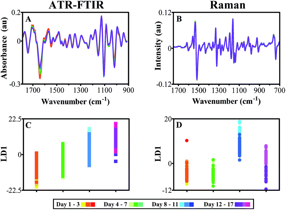 | ||
| Fig. 6 Spectra derived from ATR-FTIR (A and C) and Raman (B and D) spectroscopy with grouped time points in order to depict clear spectral differences symptomatic of leaf development. (A) ATR-FTIR pre-processed class means spectra, cut to 1800–900 cm−1, 2nd order differentiation and vector normalised; (B) Raman class means spectra cut to 1750–700 cm−1, 1st order differentiation base line correction, vector normalised and wavelet de-noised; (C) cross-validated PCA-LDA 1D scores plot of ATR-FTIR spectra against LD and (D) cross-validated PCA-LDA scores plot of Raman spectra across LD1. | ||
A number of feature extraction methods are available to feed into biomarker determination and classification models.71 In this study, three approaches are explored to ascertain robust biomarkers suggestive of standard leaf development: DBM (top panels, ○), CV approach (middle panel, □) and FFS histograms (bottom panels, Δ). In each instance, the first data group ‘Days 1–3’ was used as a reference class and any consequent changes along the biological spectrum would be indicative of developmental alterations from this starting point of spectral acquisition. The top six biomarkers for each approach were identified using a peak detection algorithm and are listed in Table 2.
| Classes | Top six discriminating biomarkers (cm−1) | |||
|---|---|---|---|---|
| DBM | CV | FFS | ||
| a Derived from one feature extraction technique. | ||||
| ATR-FTIR | Days 1–3 versus Days 4–7 | 1107 | 968 | 1192 |
| 1547 | 1057 | 1408 | ||
| 1643 | 1705 | 1327 | ||
| 1018 | 1408 | 1508 | ||
| 1126 | 1254 | 1076 | ||
| 1593 | 1512 | 1666 | ||
| Days 1–3 versus Days 8–11 | 1103 | 1331 | 1408 | |
| 1639 | 968 | 1508 | ||
| 1018 | 1057 | 1470 | ||
| 1126 | 1466 | 1358 | ||
| 1547 | 1308 | 1296 | ||
| 1593 | 1254 | 1666 | ||
| Days 1–3 versus Days 12–17 | 1639 | 1327 | 1647 | |
| 1015 | 1636 | 1751 | ||
| 1103 | 1308 | 1574 | ||
| 1123 | 1466 | 1431 | ||
| 991 | 1597 | 1099 | ||
| 1038 | 1011 | 990 | ||
| Raman | Days 1–3 versus Days 4–7 | 704 | 1318 | 1464 |
| 723 | 1173 | 1191 | ||
| 1229 | 1130 | 1654 | ||
| 1173 | 1217 | 1321 | ||
| 1103 | 1423 | 911 | ||
| 1513 | 718 | 1628 | ||
| Days 1–3 versus Days 8–11 | 1158 | 1328 | 1527 | |
| 1327 | 1157 | 1328 | ||
| 1526 | 1526 | 1157 | ||
| 1513 | 1287 | 1689 | ||
| 744 | 1186 | 1669 | ||
| 1186 | 1169 | 1643 | ||
| Days 1–3 versus Days 12–17 | 1327 | 1327 | 1326 | |
| 1513 | 1148 | 1416 | ||
| 1159 | 1598 | 1680 | ||
| 1533 | 1609 | 1624 | ||
| 744 | 1529 | 1601 | ||
| 1010 | 1510 | 1528 | ||
Initially, by comparing ‘Days 1–3’ with ‘Days 4–7’ from ATR-FTIR analysis it is clear to see a number of potential wavenumbers emerging from all three feature extraction methods (Fig. 7A). The DBM approach identifies wavenumbers principally from the protein and polysaccharide regions, emulating patterns identified in class means spectra. This is also replicated in CV and FFS analysis, additional to a number of wavenumbers across the spectrum that are also classified. Table 3 describes the top three biomarkers from each comparison, derived from wavenumbers uncovered by two or more biomarker extraction approaches, with a tentative band assignment. As shown previously, the main alterations in Fig. 7A are found at 1107 and 1408 cm−1 accounting for pectin found in the plant cell wall, as well as at ∼1510 cm−1, tentatively assigned to lignin or protein.80 Lignin is present in vascular bundles within a tomato leaf and so may be noticeable due to spectral acquisition on the leaf midrib or because of damage to the leaf surface during analysis. When comparing ‘Days 1–3’ with ‘Days 8–11’ alterations in the protein regions manifests across all three approaches with the amide III peak at 1302 cm−1 being the most discriminating (Fig. 7B). The DBM and CV methodology also show similarities in polysaccharide alterations, particularly at 1103 cm−1 associated with ester and pectins, although this is not selected by the FFS histogram. Ester bonds crosslink cutin in the leaf cuticle and thus this peak infers information about this upper leaf surface layer.83Fig. 7C illustrates parity between the DBM, CV and FFS extraction methods with each approach consistently identifying protein alterations at 1642 cm−1 the amide I peak, and carbohydrate markers at 1101 and 1014 cm−1 assigned to cellulose and pectin respectively. As this is a comparison between the two extreme time classes, the differences are expected to be more identifiable by all approaches.
 | ||
| Fig. 7 Three biomarker extraction approaches, difference between mean spectra (top panels), PCA-LDA cluster vector (middle panels) and forward feature selection histograms (bottom panels) to establish spectral biomarkers indicative of plant development in both ATR-FTIR and Raman data. ‘Days 1–3’ represent the initial spectral characterisation of the leaf and therefore ‘Days 4–7’ (A and D); ‘Days 8–11’ (B and E); and ‘Days 12–17’ (C and F) are all compared to this data class. The top six biomarkers identified in each approach are highlighted with symbols. All units are arbitrary. | ||
| Wavenumber (cm−1) | Tentative assignment | Reference | ||
|---|---|---|---|---|
| ATR-FTIR | Days 1–3 versus Days 4–7 | 1408 | CH3 deformation, νs(COO−) in pectin | 88 |
| 1512–1508 |
ν(C![[double bond, length as m-dash]](https://www.rsc.org/images/entities/char_e001.gif) C) in lignin, carotenoid or protein C) in lignin, carotenoid or protein |
43 | ||
| 1107 | ν(CO), ν(CC), pectin | 32 | ||
| Days 1–3 versus Days 8–11 | 1470–1466 | CH2 bending in lipid | 47 | |
| 1308–1296 | Amide III | 80 | ||
| 1103 | ν(C–O–C) in ester | 89 | ||
| Days 1–3 versus Days 12–17 | 1647–1636 | Amide I | 61 | |
| 1103–1099 | ν(CO) in cellulose | 36 | ||
| 1015–1013 | ν(CO), ν(CC), δ(OCH), ring in pectin | 34 | ||
| Raman | Days 1–3 versus Days 4–7 | 1229–1217 | Amide III | 55 |
| 1191–1173 | as(PO2−) in DNA | 40 | ||
| 1462 | δ(CH2) in hemicellulose | 61 | ||
| Days 1–3 versus Days 8–11 | 1158–1157 | ν(CC) in carotenoid | 90 | |
| 1328–1327 | Chlorophyll | 56 | ||
| 1526–1527 |
ν(CC) in carotenoid |
91 | ||
| Days 1–3 versus Days 12–17 | 1327–1326 | Chlorophyll | 56 | |
| 1159–1148 | ν(CC) in carotenoid | 90 | ||
| 1533–1529 |
ν(CC) in carotenoid, chlorophyll |
56 | ||
Raman data compared between ‘Days 1–3’ and ‘Days 4–7’ show very little variation, indicated by relatively noisy curves in both DBM and CV analysis and a featureless FFS histogram (Fig. 7D). As shown in ATR-FTIR data, these two data classes are most similar and therefore spectral differences would be minimal. In contrast, Fig. 7E consistently locates three distinct wavenumbers associated principally with carotenoid at 1158 and 1527 cm−1, as well as chlorophyll at 1328 cm−1. The latter of these observations may be expected as a leaf develops towards senescence, due to a breakdown of chloroplasts and therefore a decrease in chlorophyll content.84 The same wavenumbers are again deduced when comparing ‘Days 1–3’ with ‘Days 12–17’, although surprisingly these are not picked out as robustly in the FFS histogram (Fig. 7F). Alterations at the 1158 and 1526 cm−1 band begins to infer that there is a variance in carotenoid content between classes, attributed to leaf development. It is well established that carotenoid content remains constant whilst chlorophyll reduces through development of the leaf, evidenced by colour transition from green to brown in young and senescent leaves.85 Thus any alteration in carotenoids pigments is unexpected in regards to development of the leaf.
Linear regression analysis was conducted on the most distinguishing biomarkers previously determined, to ascertain any patterns in absorbance between leaves at different morphological stages (Fig. 8). In general, a negative relationship can be seen between protein absorbance over time, particularly NE leaves, typified by IR absorbance values at 1639 cm−1, representing progression from young towards senescent leaf (Fig. 8A). This is also replicated to a lesser extent in M leaves, which is attributed to the leaf being closer to senescence and therefore not experiencing as severe protein reduction in the acquisition time frame. No significant decrease in protein can be identified in S leaves over the course of the study due to already having undergone substantial protein degradation (ESI Table S5†). Fig. 8B and C highlight positive variations in absorbance bands at 1107 and 1015 cm−1 corresponding to polysaccharides cellulose and pectin, respectively. NE leaves again depict the greatest alterations at these wavenumbers corresponding to cell wall expansion. This pattern is less visible in M leaves and even less so in S leaves, mirroring the response shown in protein. A diminution of protein and increase of carbohydrate are simple characteristics of leaf development and have been effectively characterised here by ATR-FTIR in different leaf stages.
 | ||
| Fig. 8 Linear regression analysis at key biomarker wavenumbers 1639 cm−1 (A), 1103 cm−1 (B), 1015 cm−1 (C) from mean IR spectra and 1529 cm−1 (D), 1327 cm−1 (E), 1158 cm−1 (F) from mean Raman spectra of leaves at different developmental stages. | ||
Fig. 8D shows linear regression analysis of scattering intensity at 1529 cm−1 resultant from Raman analysis of NE, M and S leaves. Although only minimal significance can be seen in M leaves, there is a slight negative trend in the data, showing a reduction in chlorophyll and carotenoid intensity. This acknowledged indicator of leaf senescence appears to occur more significantly in M leaves, highlighting that chlorophyll degradation in this case appears to be a late on-set process within leaf senescence.86 In contrast, at peak 1328 cm−1 corresponding primarily with chlorophyll, no significant patterns can be identified with NE expanded leaves showing slight increases compared with small reductions in M and S leaves (Fig. 8E). Overlap with DNA and protein can be observed around this region and may contribute to masking any chlorophyll scattering effect.87 Carotenoid alterations are portrayed in Fig. 8F relative to intensity at 1158 cm−1 and do not show any significant differences between leaf samples.
Conclusion
ATR-FTIR and Raman spectroscopy are highly informative, non-destructive and robust techniques that have been limitedly employed in the field of plant science.32 Whilst many studies demonstrate the successful use of vibrational spectroscopy to characterise plant tissues in fixed and in vitro samples, thus far research has been hindered by water interference and auto-fluorescence.3 In this investigation, in vivo spectral measurements are obtained with no destructive effect on systemic plant health. Although ATR-FTIR appears to cause minor local damage, this had no significant effect on the leaf and therefore does not necessarily rule out non-destructive analysis. The technique may not be suitable for direct analysis of fruit or yieldable products, however in future field studies, a single leaf is more easily sacrificed in a plant or crop system, with no detriment to crop yield or quality. Raman spectroscopy in particular had little visible effect on plant health and viability and may prove to be a crucial tool for live plant analysis. Additionally, both complementary methods coupled with multivariate analysis, provide data that can accurately depict known plant developmental processes, providing groundwork for characterisation of complex stress responses, such as nutrient deficiency, that could be used in the field. A prerequisite for future studies would be to characterise a stress response and locate spectral biomarkers indicative of this given stress. This presents a novel method of fingerprinting plant health in a high-throughput manner, which can be effectively employed in agricultural and environmental studies.Acknowledgements
HJB is a member of the Centre for Global Eco-Innovation with ERDF funding.References
- H. C. J. Godfray, J. R. Beddington, I. R. Crute, L. Haddad, D. Lawrence, J. F. Muir, J. Pretty, S. Robinson, S. M. Thomas and C. Toulmin, Science, 2010, 327(5967), 812–818 CrossRef CAS PubMed.
- I. Domínguez-Martínez, O. G. Meza-Márquez, G. Osorio-Revilla, J. Proal-Nájera and T. Gallardo-Velázquez, J. Korean Soc. Appl. Biol. Chem., 2014, 57(1), 133–142 CrossRef.
- J. C. Mansfield, G. R. Littlejohn, M. P. Seymour, R. J. Lind, S. Perfect and J. Moger, Anal. Chem., 2013, 85(10), 5055–5063 CrossRef CAS PubMed.
- V. Llabjani, R. N. Malik, J. Trevisan, V. Hoti, J. Ukpebor, Z. K. Shinwari, C. Moeckel, K. C. Jones, R. F. Shore and F. L. Martin, Environ. Int., 2012, 48, 39–46 CrossRef CAS PubMed.
- B. E. Obinaju, A. Alaoma and F. L. Martin, Environ. Pollut., 2014, 192, 222–231 CrossRef CAS PubMed.
- M. Mecozzi, M. Pietroletti and R. Di Mento, Vib. Spectrosc., 2007, 44(2), 228–235 CrossRef CAS PubMed.
- L. G. Thygesen, M. M. Løkke, E. Micklander and S. B. Engelsen, Trends Food Sci. Technol., 2003, 14(1), 50–57 CrossRef CAS.
- D.-W. Sun, Infrared spectroscopy for food quality analysis and control, Academic Press, 2009 Search PubMed.
- M. J. Baker, J. Trevisan, P. Bassan, R. Bhargava, H. J. Butler, K. M. Dorling, P. R. Fielden, S. W. Fogarty, N. J. Fullwood, K. A. Heys, C. Hughes, P. Lasch, P. L. Martin-Hirsch, B. Obinaju, G. D. Sockalingum, J. Sulé-Suso, R. J. Strong, M. J. Walsh, B. R. Wood, P. Gardner and F. L. Martin, Nat. Protoc., 2014, 9(8), 1771–1791 CrossRef CAS PubMed.
- J. M. Chalmers, P. R. Griffiths, D. E. Pivonka, J. Chalmers and P. Griffiths, Applications of vibrational spectroscopy in pharmaceutical research and development, ed. D. E. Pivonka, J. M. Chalmers and P. R. Griffiths, 2007 Search PubMed.
- G. Clemens, J. R. Hands, K. M. Dorling and M. J. Baker, Analyst, 2014, 139(18), 4411–4444 RSC.
- P. Lasch, A. Pacifico and M. Diem, Biopolymers, 2002, 67(4–5), 335–338 CrossRef PubMed.
- M. Diem, A. Mazur, K. Lenau, J. Schubert, J. Fore, B. Bird, M. Miljković and C. Krafft, in Ex-vivo and In-vivo Optical Molecular Pathology, ed. J. Popp, 2014, ch. 3, pp. 45–102 Search PubMed.
- F. M. Lyng, E. Ó. Faoláin, J. Conroy, A. D. Meade, P. Knief, B. Duffy, M. Hunter, J. Byrne, P. Kelehan and H. J. Byrne, Exp. Mol. Pathol., 2007, 82(2), 121–129 CrossRef CAS PubMed.
- D. C. Fernandez, R. Bhargava, S. M. Hewitt and I. W. Levin, Nat. Biotechnol., 2005, 23(4), 469–474 CrossRef CAS PubMed.
- B. R. Wood, M. A. Quinn, F. R. Burden and D. McNaughton, Biospectroscopy, 1996, 2(3), 143–153 CrossRef CAS.
- P. Crow, A. Molckovsky, N. Stone, J. Uff, B. Wilson and L. Wongkeesong, Urology, 2005, 65(6), 1126–1130 CrossRef CAS PubMed.
- N. Stone and P. Matousek, Cancer Res., 2008, 68(11), 4424–4430 CrossRef CAS PubMed.
- P. Lasch, W. Haensch, D. Naumann and M. Diem, Biochim. Biophys. Acta, Mol. Basis Dis., 2004, 1688(2), 176–186 CrossRef CAS PubMed.
- M. K. Kuimova, K. Chan and S. G. Kazarian, Appl. Spectrosc., 2009, 63(2), 164–171 CrossRef CAS PubMed.
- J. Ollesch, M. Heinze, H. M. Heise, T. Behrens, T. Brüning and K. Gerwert, J. Biophotonics, 2014, 7(3–4), 210–221 CrossRef CAS PubMed.
- K. M. Dorling and M. J. Baker, Trends Biotechnol., 2013, 31(6), 327–328 CrossRef CAS PubMed.
- D. Lin, S. Feng, J. Pan, Y. Chen, J. Lin, G. Chen, S. Xie, H. Zeng and R. Chen, Opt. Express, 2011, 19(14), 13565–13577 CrossRef CAS PubMed.
- J. W. Allwood, J. Heald, A. J. Lloyd, R. Goodacre and L. A. Mur, in Plant Metabolomics, Springer, 2012, vol. 860, pp. 31–49 Search PubMed.
- M. Baranska, W. Schütze and H. Schulz, Anal. Chem., 2006, 78(24), 8456–8461 CrossRef CAS PubMed.
- D. Gill, R. Kilponen and L. Rimai, Nature, 1970, 227(5259), 743–744 CrossRef CAS.
- R. H. Wilson, A. C. Smith, M. Kačuráková, P. K. Saunders, N. Wellner and K. W. Waldron, Plant Physiol., 2000, 124(1), 397–406 CrossRef CAS PubMed.
- H. E. Johnson, D. Broadhurst, R. Goodacre and A. R. Smith, Phytochemistry, 2003, 62(6), 919–928 CrossRef CAS.
- Z. Wei, L. Dong and Z. Tian, Pak. J. Bot., 2009, 41(4), 1743–1750 CAS.
- P. Griffiths and J. A. De Haseth, Fourier transform infrared spectrometry, Wiley-Interscience, 2007 Search PubMed.
- F. L. Martin, Nat. Methods, 2011, 8(5), 385–387 CrossRef CAS PubMed.
- H. Schulz and M. Baranska, Vib. Spectrosc., 2007, 43(1), 13–25 CrossRef CAS PubMed.
- Y. Li, D. Kong and H. Wu, Ind. Crops Prod., 2013, 41(1), 269–278 CrossRef CAS PubMed.
- M. Kacurakova, P. Capek, V. Sasinkova, N. Wellner and A. Ebringerova, Carbohydr. Polym., 2000, 43(2), 195–203 CrossRef CAS.
- P. Rösch, W. Kiefer and J. Popp, Biopolymers, 2002, 67(4–5), 358–361 CrossRef PubMed.
- M. C. McCann, M. Defernez, B. R. Urbanowicz, J. C. Tewari, T. Langewisch, A. Olek, B. Wells, R. H. Wilson and N. C. Carpita, Plant Physiol., 2007, 143(3), 1314–1326 CrossRef CAS PubMed.
- M. McCann, L. Chen, K. Roberts, E. Kemsley, C. Sene, N. Carpita, N. Stacey and R. Wilson, Physiol. Plant., 1997, 100(3), 729–738 CrossRef CAS PubMed.
- D. Harris, V. Bulone, S.-Y. Ding and S. DeBolt, Plant Physiol., 2010, 153(2), 420–426 CrossRef CAS PubMed.
- R. Gessner, P. Rösch, R. Petry, M. Schmitt, M. Strehle, W. Kiefer and J. Popp, Analyst, 2004, 129(12), 1193–1199 RSC.
- E. Gidman, R. Goodacre, B. Emmett, A. R. Smith and D. Gwynn-Jones, Phytochemistry, 2003, 63(6), 705–710 CrossRef CAS.
- J. W. Allwood, D. I. Ellis and R. Goodacre, Physiol. Plant., 2008, 132(2), 117–135 CAS.
- P. Heraud, S. Caine, G. Sanson, R. Gleadow, B. R. Wood and D. McNaughton, New Phytol., 2007, 173(1), 216–225 CrossRef PubMed.
- P. Yu, J. J. McKinnon, C. R. Christensen, D. A. Christensen, N. S. Marinkovic and L. M. Miller, J. Agric. Food Chem., 2003, 51(20), 6062–6067 CrossRef CAS PubMed.
- B. O. Budevska, S. T. Sum and T. J. Jones, Appl. Spectrosc., 2003, 57(2), 124–131 CrossRef CAS PubMed.
- D. S. Himmelsbach, S. Khalili and D. E. Akin, J. Sci. Food Agric., 2002, 82(7), 685–696 CrossRef CAS PubMed.
- F. Monti, R. Dell'Anna, A. Sanson, M. Fasoli, M. Pezzotti and S. Zenoni, Vib. Spectrosc., 2012, 65, 36–43 CrossRef PubMed.
- B. Ribeiro da Luz, New Phytol., 2006, 172(2), 305–318 CrossRef CAS PubMed.
- D. G. Ivanova and B. R. Singh, Biopolymers, 2003, 72(2), 79–85 CrossRef CAS PubMed.
- E. Dubis, A. Dubis and J. Morzycki, J. Mol. Struct., 1999, 511, 173–179 CrossRef.
- E. N. Dubis, A. T. Dubis and J. Popławski, J. Mol. Struct., 2001, 596(1), 83–88 CrossRef CAS.
- E. B. Wilson, Molecular vibrations: the theory of infrared and Raman vibrational spectra, Courier Dover Publications, 1955 Search PubMed.
- E. Smith and G. Dent, Modern Raman spectroscopy: a practical approach, John Wiley & Sons, 2005 Search PubMed.
- M. Baranska, M. Roman, H. Schulz and R. Baranski, Curr. Anal. Chem., 2013, 9(1), 108–127 CrossRef CAS.
- B. Schrader, A. Hoffmann and S. Keller, Spectrochim. Acta, Part A, 1991, 47(9), 1135–1148 CrossRef.
- C. Sene, M. C. McCann, R. H. Wilson and R. Grinter, Plant Physiol., 1994, 106(4), 1623–1631 CAS.
- L. Zeiri, J. Raman Spectrosc., 2007, 38(7), 950–955 CrossRef CAS PubMed.
- P. Rösch, J. Popp and W. Kiefer, J. Mol. Struct., 1999, 480–481, 121–124 CrossRef.
- J. C. Merlin, Pure Appl. Chem., 1985, 57(5), 785–792 CrossRef CAS.
- Y. Zeng, M. E. Himmel and S.-Y. Ding, in Biomass Conversion, Springer, Methods in Molecular Biology, 2012, vol. 908, pp. 49–60 Search PubMed.
- Y. Zeng, B. G. Saar, M. G. Friedrich, F. Chen, Y.-S. Liu, R. A. Dixon, M. E. Himmel, X. S. Xie and S.-Y. Ding, BioEnergy Res., 2010, 3(3), 272–277 CrossRef.
- M. Chylinska, M. Szymanska-Chargot and A. Zdunek, Plant Methods, 2014, 10(1), 14 CrossRef PubMed.
- R. Picorel, G. Chumanov, E. Torrado, T. M. Cotton and M. Seibert, J. Phys. Chem. B, 1998, 102(15), 2609–2613 CrossRef CAS.
- M. Seibert, R. Picorel, J.-H. Kim and T. M. Cotton, Methods Enzymol., 1992, 213, 31–42 CAS.
- B. Schrader, Infrared and Raman spectroscopy: methods and applications, John Wiley & Sons, 2008 Search PubMed.
- F. L. Martin, J. G. Kelly, V. Llabjani, P. L. Martin-Hirsch, I. I. Patel, J. Trevisan, N. J. Fullwood and M. J. Walsh, Nat. Protoc., 2010, 5(11), 1748–1760 CrossRef CAS PubMed.
- J. Trevisan, P. P. Angelov, A. D. Scott, P. L. Carmichael and F. L. Martin, Bioinformatics, 2013, 29(8), 1095–1097 CrossRef CAS PubMed.
- E. Domínguez, J. A. Heredia-Guerrero and A. Heredia, New Phytol., 2011, 189(4), 938–949 CrossRef PubMed.
- M. Riederer and L. Schreiber, J. Exp. Bot., 2001, 52(363), 2023–2032 CrossRef CAS.
- G. Strang and T. Nguyen, Wavelets and filter banks, SIAM, 1996 Search PubMed.
- P. Matousek, Chem. Soc. Rev., 2007, 36(8), 1292–1304 RSC.
- J. Trevisan, P. P. Angelov, P. L. Carmichael, A. D. Scott and F. L. Martin, Analyst, 2012, 137(14), 3202–3215 RSC.
- I. I. Patel, W. J. Harrison, J. G. Kerns, J. Filik, K. Wehbe, P. L. Carmichael, A. D. Scott, M. P. Philpott, M. D. Frogley, G. Cinque and F. L. Martin, Anal. Bioanal. Chem., 2012, 404(6–7), 1745–1758 CrossRef CAS PubMed.
- F. L. Martin, M. J. German, E. Wit, T. Fearn, N. Ragavan and H. M. Pollock, J. Comput. Biol., 2007, 14(9), 1176–1184 CrossRef CAS PubMed.
- J. Trevisan, P. P. Angelov, I. I. Patel, G. M. Najand, K. T. Cheung, V. Llabjani, H. M. Pollock, S. W. Bruce, K. Pant and P. L. Carmichael, Analyst, 2010, 135(12), 3266–3272 RSC.
- J. G. Kelly, J. l. Trevisan, A. D. Scott, P. L. Carmichael, H. M. Pollock, P. L. Martin-Hirsch and F. L. Martin, J. Proteome Res., 2011, 10(4), 1437–1448 CrossRef CAS PubMed.
- J. Trevisan, J. Park, P. P. Angelov, A. A. Ahmadzai, K. Gajjar, A. D. Scott, P. L. Carmichael and F. L. Martin, J. Biophotonics, 2014, 7(3–4), 254–265 CrossRef CAS PubMed.
- K. R. Coombes, H. A. Fritsche, C. Clarke, J.-N. Chen, K. A. Baggerly, J. S. Morris, L.-C. Xiao, M.-C. Hung and H. M. Kuerer, Clin. Chem., 2003, 49(10), 1615–1623 CAS.
- I. Weissflog, N. Vogler, D. Akimov, A. Dellith, D. Schachtschabel, A. Svatos, W. Boland, B. Dietzek and J. Popp, Plant Physiol., 2010, 154(2), 604–610 CrossRef CAS PubMed.
- D. J. Cosgrove, Nat. Rev. Mol. Cell Biol., 2005, 6(11), 850–861 CrossRef CAS PubMed.
- Z. Movasaghi, S. Rehman and D. I. ur Rehman, Appl. Spectrosc. Rev., 2008, 43(2), 134–179 CrossRef CAS.
- C. M. Smart, New Phytol., 1994, 126(3), 419–448 CrossRef CAS PubMed.
- V. Buchanan-Wollaston, J. Exp. Bot., 1997, 48(2), 181–199 CrossRef PubMed.
- P. Kolattukudy, K. Espelie and C. Soliday, in Plant Carbohydrates II, Springer, 1981, pp. 225–254 Search PubMed.
- B. Schrader, B. Dippel, I. Erb, S. Keller, T. Löchte, H. Schulz, E. Tatsch and S. Wessel, J. Mol. Struct., 1999, 480–481, 21–32 CrossRef CAS.
- R. Baranski, M. Baranska and H. Schulz, Planta, 2005, 222(3), 448–457 CrossRef CAS PubMed.
- L. Guyer, S. S. Hofstetter, B. Christ, B. S. Lira, M. Rossi and S. Hörtensteiner, Plant Physiol., 2014, 166(1), 44–56 CrossRef CAS PubMed.
- Z. Movasaghi, S. Rehman and I. U. Rehman, Appl. Spectrosc. Rev., 2007, 42(5), 493–541 CrossRef CAS.
- L. Chen, N. C. Carpita, W.-D. Reiter, R. H. Wilson, C. Jeffries and M. C. McCann, Plant J., 1998, 16(3), 385–392 CrossRef CAS.
- R. Hunt, Basic growth analysis, Unwin Hyman Ltd, 1990 Search PubMed.
- H. Schulz, M. Baranska and R. Baranski, Biopolymers, 2005, 77(4), 212–221 CrossRef CAS PubMed.
- J. J. Jansen, J. W. Allwood, E. Marsden-Edwards, W. H. van der Putten, R. Goodacre and N. M. van Dam, Metabolomics, 2009, 5(1), 150–161 CrossRef CAS.
Footnote |
| † Electronic supplementary information (ESI) available. See DOI: 10.1039/c5ay00377f |
| This journal is © The Royal Society of Chemistry 2015 |