
 Open Access Article
 This Open Access Article is licensed under a
 Creative Commons Attribution 3.0 Unported Licence
Making colourful sense of Raman images of single cells†
Lorna
Ashton
*ab,
Katherine A.
Hollywood
ac and
Royston
Goodacre
a
aManchester Institute of Biotechnology, University of Manchester, 131, Princess Street, Manchester, M1 7DN, UK. E-mail: l.ashton@lancaster.ac.uk
bDepartment of Chemistry, Faraday Building, Lancaster University, Lancaster, LA1 4YB, UK
cFaculty of Life Science, University of Manchester, Manchester, M13 9PT, UK
First published on 3rd February 2015
Abstract
In order to understand biological systems it is important to gain pertinent information on the spatial localisation of chemicals within cells. With the relatively recent advent of high-resolution chemical imaging this is being realised and one rapidly developing area of research is the Raman mapping of single cells, an approach whose success has vast potential for numerous areas of biomedical research. However, there is a danger of undermining the potential routine use of Raman mapping due to a lack of consistency and transparency in the way false-shaded Raman images are constructed. In this study we demonstrate, through the use of simulated data and real Raman maps of single human keratinocyte (HaCaT) cells, how changes in the application of colour shading can dramatically alter the final Raman images. In order to avoid ambiguity and potential subjectivity in image interpretation we suggest that data distribution plots are used to aid shading approaches and that extreme care is taken to use the most appropriate false-shading for the biomedical question under investigation.
Introduction
Raman mapping is a powerful technique for single cell analysis, providing vast amounts of spatially resolved biochemical data from which cellular composition and sub-cellular components can be identified.2–4 A single Raman spectrum from a cell can supply detailed information on molecular constituents including proteins (amino acid and conformational structures), nucleic acids (DNA and RNA) and lipids (cholesterol and CH2 groups).4–7 Due to the vast and continuing improvements in Raman instrumentation, including high quality lasers, CCD cameras and optical elements, whole cells can now be successfully mapped within minutes with thousands of Raman spectra being acquired in 0.5–1 μm steps. The importance of single cell analysis for many areas of biomedical research, including cell biology, neurobiology, pharmacology and developmental biology means that the label-free, non-destructive technique of Raman imaging, with the tantalising potential of live cell imaging, has a pivotal role in the future of single cell imaging.8The successful construction of a Raman map requires the generation of a false-colour image in which each pixel is shaded according to the relative intensities of the defined Raman spectral regions or peaks or specific components such as principal component scores from principal component analysis. This shading across the full Raman map can then be used to resolve spatially the distribution of these specific features within the cell (e.g. nucleus from cytoplasm) and thus conclusions can be drawn from the various shades or colours. However, standards for the way this shading is applied are presently lacking in Raman imaging and this lack of objectivity means there is very real potential that if false-colouring is not carefully carried out data may be over-interpreted or important details may be inadvertently missed.9,10 Frequently, default settings in imaging software are applied without questioning if this is the most appropriate approach, or in the very worst situations shading is ‘randomly’ adjusted to give the most pleasing image without any consideration for the biochemical implications. In this paper we will demonstrate through the use of simulated data and single cell Raman maps of HaCaT cells (before and after drug treatment) the potential effects of changing shading parameters and how care needs to be taken in the application of false-shading for appropriate interpretation of Raman generated chemical images.
Materials and methods
Cell culture
Drug compounds and cell culture reagents were purchased from Sigma Aldrich (Gillingham, UK) unless otherwise stated. HaCaT cells11 were routinely cultured in 75 cm2 culture flasks with Dulbecco's Modified Eagle Medium (DMEM) supplemented with 10% Foetal Bovine Serum (FBS) and 1% penicillin-streptomycin. To avoid any bias associated with the undefined nature of FBS, a single batch was used for all experiments described within.Cells were grown to ∼90% confluency, after which they were detached from the cell culture flask using trypsin-EDTA. The cells were then seeded at ∼30![[thin space (1/6-em)]](https://www.rsc.org/images/entities/char_2009.gif) 000 cells onto a sterile CaF2 Raman compatible window within 35 mm culture dishes.
000 cells onto a sterile CaF2 Raman compatible window within 35 mm culture dishes.
Drug preparation
A stock solution of dithranol was freshly prepared in acetone prior to use. An initial stock solution of 1 mg mL−1 was prepared followed by serial dilution with DMEM medium to a concentration of 2 μM, as this concentration can still be clinically effective but has been shown not to induce apoptosis.12 We ensured that the drug was prepared and that subsequent solutions were kept in dark conditions to avoid degradation.Drug treatment
The HaCaT cells were cultured under normal conditions for 24 h to allow the cells to adhere and undergo normal cell growth. After 24 h a complete medium change was conducted before treatment with 2 μM of dithranol. Control dishes were also prepared by either conducting a complete medium change only (untreated control) or by the addition of an equivalent volume of acetone (vehicle control).HaCaT cells were then incubated with dithranol for 2, 6, 12, 16 and 22 h respectively. At each collection time point the cells were washed twice with phosphate buffered saline (PBS) before fixing with methanol (100%, −20 °C, 5 min). Cells were examined before and after fixing to ensure no obvious changes in structure. The CaF2 discs with cells were then washed again with PBS and stored in PBS at 4 °C until analysis. Control cells were fixed after 22 h and processed as previous.
Raman spectroscopy
All Raman spectra were collected using a confocal Raman system (inVia, Renishaw plc, Wotton-Under-Edge, UK) coupled to a 785 nm wavelength laser. StreamLineHR mapping (which uses a laser-spot focus) was carried out using a 60× NA = 1.00 water immersion objective (LUMPLFLN 60XW Olympus) in high confocal mode, at a step size of 1 μm. A power intensity of ∼30 mW on the sample and an exposure time of 1 s was applied, with the exception of the untreated cell Raman map (Fig. 1–3) where an exposure time of 5 s was used. The average total collection time for a complete cell was ∼25 min. | ||
| Fig. 1 False-coloured Raman images of a single HaCaT cell. Rainbow colour shading is relative to peak area intensity in the regions of (A) 1600–1700 cm−1, (B) 990–1010 cm−1, (C) 768–800 cm−1 and 693–713 cm−1 as shaded in the example Raman spectrum (E) taken from a central pixel of the Raman map. | ||
 | ||
| Fig. 2 An overlaid Raman image of a single HaCaT cell. Red shading represents the peak intensity at 990–1010 cm−1, yellow shading represents peak intensity at 768–800 cm−1 and white shading represents peak intensity at 693–713 cm−1. | ||
 | ||
| Fig. 3 A comparison of overlaid and individual Raman images constructed from a single Raman map of a fixed HaCaT cell using various intensity ranges and colour ramps. (A) Shading over the minimum to maximum peak area intensity range, (B) shading over the 5–95% peak area intensity range, (C) shading based on an arbitrarily chosen peak area intensity range and (D) shading from 0–maximum peak area intensity range but with a steeper change in colour ramp. All red shading represents the peak intensity at 990–1010 cm−1, yellow shading peak intensity at 768–800 cm−1 and white shading peak intensity at 693–713 cm−1. Colour bars are shown to the right of each image. | ||
Data analysis
Raman maps were smoothed using the noise filter feature within Wire 4.0 (the instrument control software) with a setting of 5 components. Peak areas were calculated in Wire 4.0 and exported to MATLAB software version 2011a for generation of Raman images and distribution plots (The MathWorks, MA, USA). Overlaid images were constructed in ImageJ (http://imagej.nih.gov/ij) from the original images created in MATLAB.Simulated data were generated from a hand-drawn picture which was divided into 70 × 50 pixels and an appropriate value between 0 and 6000 was given to each pixel so that the picture could then be displayed as a false-shaded 2D map using MATLAB.
Results and discussion
Raman images
In order to construct an image from a Raman map, where each spectrum relates to a single pixel, a value for each spectrum such as the Raman intensity of a defined spectral region must to be represented by a false-colour scale. Often, the first step in producing a Raman image of a single cell is to shade to the peak intensity of a representative spectral region such as the amide I (1600–1700 cm−1). This approach enables the identification of protein material, most often associated with the cytoplasm, and can therefore be used to define the outline of the cell, as demonstrated in Fig. 1A for the Raman map of a HaCaT cell. Specific Raman peaks can also be selected such as the peaks at ∼1004 cm−1 (Fig. 1B), ∼780 cm−1 (Fig. 1C) and ∼703 cm−1 (Fig. 1D) assigned to phenylalanine (Phe),4–6 nucleic acids (NA)5–7 and lipids,5 respectively. For each of these Raman images the peak areas were calculated from the signal to baseline (using Wire 4.0) for a defined spectral region as shaded in the example cell spectrum (Fig. 1E): 1600–1700 for the amide I peak, 990–1010 cm−1 for the 1004 cm−1 peak, 768–800 for the 780 cm−1 peak and 693–713 cm−1 for the 703 cm−1 peak.The Raman images in Fig. 1 have been false-shaded using a rainbow scale, which is frequently the default setting in many software packages, with pixel shading relative to the values shown on the colour bar to the right of the image. Clear differences can be observed between each image constructed from the different features in the Raman map of the HaCaT cell; however, for presentation purposes one single image is usually preferred with each feature shaded a different colour and then overlaid (Fig. 2). Interpolation, which can be used to estimate an image value at a location between pixels thereby softening the edges of the pixel has also been applied in Fig. 2 (using the MATLAB function interp) thereby further improving the appearance of the image. This single image approach not only saves space, reducing the number of figures needed for publication with a visibly more pleasing image but, can also reveal subtle differences between spatial patterns. The difficulty is that in order to create an impressive overlaid image the shading or colour ramps often need to be extensively altered for each individual image.
The choice of intensity range applied to individual images, such as min–max or 5–95%, can often result in one or two features dominating over the other features in the overlaid image resultantly obscuring important information. For example in Fig. 3A and B the Raman images constructed from the peak areas at 703 and 780 cm−1 dominate over the image constructed from the peak area at 1004 cm−1. One way to ensure that all three features can be observed in the overlaid image is to arbitrarily alter the intensity ranges (Fig. 3C). When the range of intensity values for the peak at 1004 cm−1 are changed from a min–max of 20–200 counts to a much narrower range of 25–80 counts (with all pixels of values below 25 counts shaded black and any pixels above 80 counts shaded red) the Phe features become clearer in the overlaid image. Alternatively, the actual colour ramps can be altered as demonstrated in Fig. 3D where the intensity range of 0–max has been used for all three images but the colour ramps have been subjectively adjusted to give the ‘best’ image, which is also the original image displayed in Fig. 2. The significant change in the images depending on shading choice raises the question of what approach should be taken when deciding on appropriate colour ranges and ramps for single cell analysis? A further example of the importance of shading ranges is given using simulated maps (Fig. 4).
 | ||
| Fig. 4 A comparison of rainbow shaded images constructed from a simulated Raman map with an intensity range of (A) 500–2000 counts, (B) 500–3500 counts, (C) minimum to maximum intensity and (D) minimum to maximum intensity but using discrete colours to form the colour ramp, (i) and (ii) identify the position of the bird shapes. Colour bars are shown to the left of each image. | ||
Simulated images
In Fig. 4A a rainbow colour ramp from 500 to 2000 counts has been applied to the simulated peak intensity data resulting in an image of a horse, however, when the intensity range is increased to 3500 counts (Fig. 4B) the new image reveals stripes showing that the image is not of a horse but is indeed a zebra. From Fig. 4A and B alone it is not possible to know what the chosen intensity ranges actually relate to, whether it is the min–max intensity, 5–95% intensity or some other arbitrary chosen range, whereas the additional labelling in Fig. 4C reveals that the full intensity range is from 0 to 6000 counts. These differences highlight the importance of extensive labelling of colour bars relative to the full intensity range rather than merely showing arbitrary numbers, which in isolation can become meaningless. Furthermore, when the full intensity range is used not only can a zebra be seen in the image but also the shape of a bird (highlighted in yellow) perched on the back of the zebra (Fig. 4C). Despite Fig. 4A, 4B and 4C looking significantly different none are actually incorrect they just reveal different information. If the question being asked is whether or not the image is of an animal than Fig. 4A is sufficient to answer it and if the question is what kind of animal is present, then Fig. 4B is required. However, if the question is addressing how many animal shapes are visible then the intensity range and colour ramp have to be more carefully chosen. The simulated data set displayed in Fig. 4 was specifically designed to display two birds on the zebra's back; one formed by intensities in the range of 3400–4000 counts (Fig. 4D (i)) and a second in the range of 5200–6000 counts (Fig. 4D (ii)). Only in Fig. 4D when the colour ramp has been replaced with discrete colours can the second bird shape (this time highlighted in red) be observed despite the fact that these pixels are of the highest intensity. It is well documented that a major disadvantage of using a rainbow scale is that it draws attention to the yellow colour despite this being of a lower value than anything shaded in dark red9,10,13 and hence the second bird is difficult to see in Fig. 4C. Rainbow shading is also reported as being unfriendly to people with any form of colour-blindness;10,13 consequently, despite being one of the most commonly used colour ramps, rainbow shading is something that should be avoided. What Fig. 4 does demonstrate is that the intensity ranges and colour ramps need to be carefully chosen to display the most appropriate information.Dithranol uptake in HaCaT cells
The choice of shading parameters is paramount for studies that require the comparison of different Raman images, for example in investigating the uptake of a drug by single cells.Fig. 5 compares the Raman images of HaCaT cells fixed 16 hours post treatment with the anti-psoriasis drug dithranol, constructed from the peak area at 598–653 cm−1 associated with the presence of dithranol (see ESI† and Fig. S1 and S2). Clear differences can again be observed between the images depending on the colour ramp used. However, as well as displaying the standard colour bar for each image, we also show the colour ramp overlaid onto the distribution plot of all the peak area intensity values calculated from the Raman map (the grey square highlights the different intensity ranges used to construct each map). It can be observed in the distribution plot for the peak area from 598–653 cm−1 that the majority of values are actually 0 or less. When a colour ramp from min–max intensity is used (Fig. 5A) the lighter grey shading actually starts below 0 and results in the appearance of dithranol outside of the fixed cell despite being washed twice in PBS before fixing. These negative values are due to noise in the spectrum creating a small negative peak when a baseline is drawn between the two points and hence any values below 0 should be disregarded in the map. It is also important to note that because of the large ratio of background to cellular material in the Raman map when a 5–95% colour ramp is applied some of the lighter shaded values still fall below zero (Fig. 5B). An alternative approach is to shade only the highest values, particularly as the aim of this study was to monitor regions of highest dithranol uptake within the cells, nevertheless, this still requires a decision to be made as to what should be classed as a high value (Fig. 5C). Of the four images constructed from the Raman map Fig. 5D looks the most reliable as no dithranol can be observed outside of the cells and a good distribution can be seen inside the cells. This choice of shading results in a colour ramp from 0–16 as all pixels of a value below zero are shaded black and above 16 are shaded white. If this colour ramp is only shown as a colour bar from 0–16 it may be misleading as many of actual pixels shaded white are of much higher intensity than 16 and, as previously discussed, without further labelling there is no relative meaning attributed to these numbers. However, by examining the distribution plot before shading, not only can a more objective decision be made as to what is the most appropriate colour ramp to apply (rather than simply using default min–max intensities, set percentages such as 5–95% or at worst adjusting the shading until it looks nice) but the final choice can also be observed relative to the full range and distribution of peak area values.
 | ||
| Fig. 5 A comparison of Raman images constructed from a Raman map of two HaCaT cells fixed 16 h after treatment with dithranol. Grey shading is relative to the peak area 598–653 cm−1 assigned to dithranol (see ESI†) and images are shaded to a peak area intensity range of (A) minimum to maximum, (B) 5–95%, (C) 15–40 counts and (D) 0–16 counts. Standard colour bars are shown to the right of each image along with a distribution plot of all the peak area values overlaid with the colour ramp. The grey box indicates the intensity range used to construct each image. | ||
It is very difficult to have exactly the same response for two Raman maps. This may be due to sample thickness differences, distribution of molecules, or the laser fluency. All of which are important when the pixel size is ca. 1 μm and therefore the voxel volume is only ca. 1 pL. Thus a consistent choice of shading is extremely important when comparing overlaid Raman images constructed from Raman maps collected at varying times or conditions, as in the case of HaCaT cells fixed at different time points after treatment with dithranol (Fig. 6). Although care was taken to optimise spectral collection before all Raman mapping it is often difficult to obtain a consistent quality of Raman maps not only due to instrumental differences but also variation in the quality of fixing techniques and the integrity of the individual cells, all of which can change throughout an experiment. Different peak area intensity values can clearly be observed between Raman maps. For the peak area of the Phe assigned peak at ∼1004 cm−1 a maximum intensity of ∼140 counts is reached in the Raman map of the cells fixed after 2 h (Fig. 6A) compared to only a maximum of 60 counts for the Raman map of the cells fixed 22 h after treatment (Fig. 6D). Furthermore, the shape of distribution of the peak area intensity values also varies significantly between Raman maps, and consequently, both the shape and intensity ranges need to be taken into account when applying colour ramp to the Raman images. In Fig. 6, for all the Raman images the overall distribution was used as a guide to the appropriate application of each colour ramp, keeping a consistent approach throughout. In the case of the peak area values for dithranol only, the highest intensity values were shaded from grey to white. From the white shading in the Raman images it can be observed that from 0–6 h the drug remains in the outer region of the cells moving further into the cells 12 h after treatment. This is consistent with previous reports that suggest that dithranol-induced apoptotic events in HaCaT cells occur from 6–24 h exposure.12
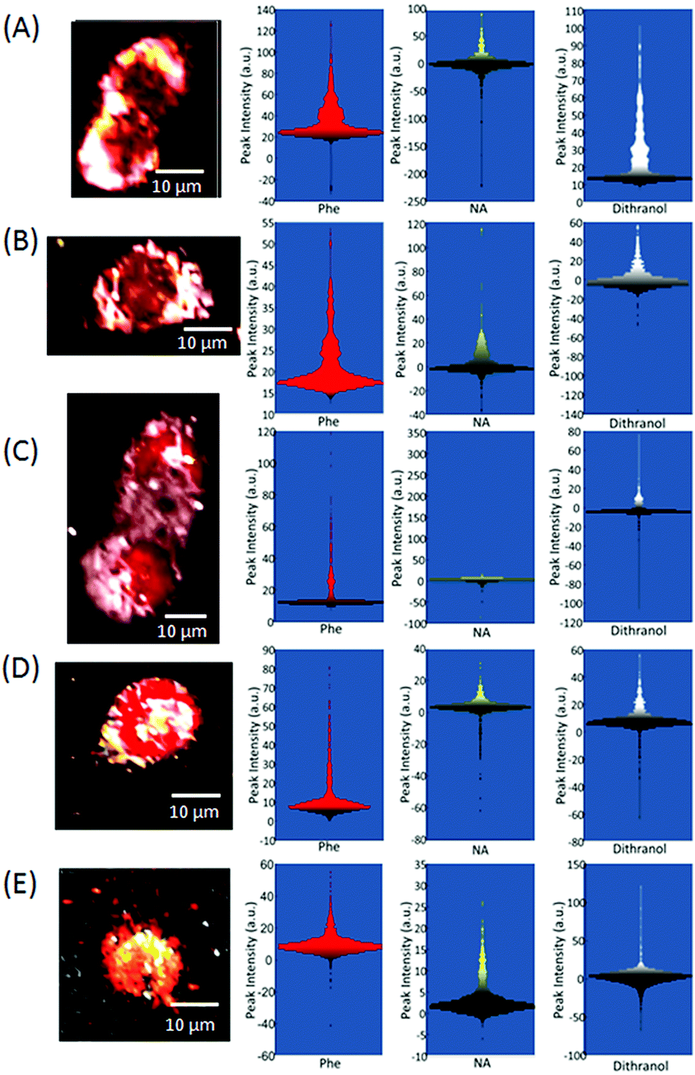 | ||
| Fig. 6 A comparison of overlaid Raman images constructed from Raman maps of HaCaT cells fixed (A) 2 h, (B) 6 h, (C) 12 h, (D) 16 h and (E) 22 h after treatment with dithranol. All red shading represents the peak intensity at 990–1010 cm−1 (phenylalanine, Phe), yellow shading peak intensity at 768–800 cm−1 (nucleic acids, NA) and white shading peak intensity at 598–653 cm−1 (dithranol). The distribution plots overlaid with the colour ramps used to construct the images are also shown for the three regions. | ||
Conclusions
Although Raman mapping is increasing in popularity and is a powerful technique for single cell analysis, providing chemical, biomolecular and spatial information, Raman false-shaded images need to be very carefully constructed. As demonstrated in this paper, the final image can vary dramatically depending on both the range of intensities and the colour ramp used in the image, particularly when several images are overlaid. First, the choice of shading needs to be applicable to the system under investigation. If the whole cell composition is to be investigated then the full intensity range from 0 to maximum intensity is usually required to provide the greatest detail. If a specific component is to be tracked, as in the uptake of dithranol by HaCaT cells, then a small intensity range or a steeper colour ramp may be more applicable. Second, and more importantly, no matter what shading parameters are used the details of these need to be made available. If Raman imaging of single cells is to become a routinely accepted technique then a transparency in the procedures used is essential. Showing simple colour bars with arbitrary numbers does not provide any useful information as to how a Raman image has been constructed, which is essential if other researchers are to be able to reproduce the data shown. However, if the distribution plot is also provided, then the choice of colour ramp relative to intensity values and distribution can be more easily assessed. We also show that with careful shading, Raman images of HaCaT cells treated with dithranol and fixed at different time points clearly reveal changes in the location of dithranol within the cell over time thus illustrating the power of Raman imaging for assessing the distribution of drugs in cells without recourse to labelling the target molecule of interest, which may of course alter its physical and chemical properties and hence interaction with its mode- and site-of-action.Acknowledgements
All authors thank BBSRC for support both from BRIC (BB/G010250/1; BB/K011170/1) and sLoLa (BB/K00199X/1) programmes. Others: We thank Prof. Anna Nicolaou and Dr Magdalena Kiezel from Manchester Pharmacy School, The University of Manchester for kind provision of the HaCaT cells. We thank Katherine Lau from Renishaw for useful discussions on Raman imaging.References
- K. Klein, A. M. Gigler, T. Aschenbrenne, R. Monetti, W. Bunk, F. Jamitzky, G. Morfill, R. W. Stark and J. Schlegel, Biophys. J., 2012, 102, 360–368 CrossRef CAS PubMed.
- D. H. Kim, R. M. Jarvis, J. W. Allwood, G. Batman, R. E. Moore, E. Marsden-Edwards, L. Hampson, I. N. Hampson and R. Goodacre, Anal. Bioanal. Chem., 2010, 398, 3051–3061 CrossRef CAS PubMed.
- A. Ghita, F. C. Pascut, M. Mather, V. Sottile and I. Notingher, Anal. Chem., 2012, 84, 3155–3162 CrossRef CAS PubMed.
- A. F. Palonpon, M. Sodeoka and K. Fujita, Curr. Opin. Chem. Biol., 2013, 708–715 CrossRef CAS PubMed.
- V. V. Pully, A. T. M. Lenferink and C. Otto, J. Raman Spectrosc., 2011, 42, 167–173 CrossRef CAS.
- Q. Matthews, A. Jirasek, J. J. Lum and A. G. Brolo, Phys. Med. Biol., 2011, 56, 6839–6855 CrossRef CAS PubMed.
- F. C. Pascut, S. Kalra, V. George, N. Welch, C. Denning and I. Notingher, Biochim. Biophys. Acta, Gen. Subj., 2013, 1830, 3517–3524 CrossRef CAS PubMed.
- D. I. Ellis, D. P. Cowcher, L. Ashton, S. O'Hagan and R. Goodacre, Analyst, 2013, 138, 3871–3884 RSC.
- B. E. Rogowitz and L. A. Treinish, IEEE Spectrum, 1998, 35, 52–59 CrossRef.
- D. Borland and R. M. Taylor, IEEE Comput. Graphics Appl., 2007, 14–17 CrossRef.
- P. Boukamp, R. T. Petrussevska, D. Breitkreutz, J. Hornung, A. Markham and N. E. Fusenig, J. Cell Biol., 1988, 106, 761–771 CrossRef CAS.
- S. E. George, R. J. Anderson, M. Haswell and P. W. Groundwater, J. Pharm. Pharmacol., 2013, 552–560 CrossRef CAS PubMed.
- A. Light and P. J. Bartlein, EOS Trans., Am. Geophys. Unioin, 2004, 85, 385–391 CrossRef.
Footnote |
| † Electronic supplementary information (ESI) available. See DOI: 10.1039/c4an02298j |
| This journal is © The Royal Society of Chemistry 2015 |