Baseline correction using asymmetrically reweighted penalized least squares smoothing

Abstract

Baseline correction methods based on penalized least squares are successfully applied to various spectral analyses. The methods change the weights iteratively by estimating a baseline. If a signal is below a previously fitted baseline, large weight is given. On the other hand, no weight or small weight is given when a signal is above a fitted baseline as it could be assumed to be a part of the peak. As noise is distributed above the baseline as well as below the baseline, however, it is desirable to give the same or similar weights in either case. For the purpose, we propose a new weighting scheme based on the generalized logistic function. The proposed method estimates the noise level iteratively and adjusts the weights correspondingly. According to the experimental results with simulated spectra and measured Raman spectra, the proposed method outperforms the existing methods for baseline correction and peak height estimation.

---

1. Introduction

Spectroscopies such as infrared spectroscopy and Raman spectroscopy are being increasingly used to measure, both directly and indirectly, a large number of chemical and physical properties of materials. Spectral interference, including varying backgrounds and noise, leads to problems with instrument calibration and quantization of spectral information. According to previous studies, one of the most significant sources of spectral variation is a curved background mainly caused by fluorescence. Hence, background elimination or baseline correction for spectral data has been paid much attention and several methods have been proposed.^1–4

The diverse sources of background and additive noise make it hard to correct baseline for experimental spectral data. Furthermore as a baseline is usually varying from sample to sample, the situation is much worse. Wavelet transform was introduced to eliminate the varying background.^5–7 As the method relies on the filtering capabilities of wavelet transform, a baseline should be well-separated in the transform domain. But real world signals often collide with this hypothesis. Moreover, it is rather complex to implement due to wavelet transform or related optimization.

A method without special assumption was proposed for baseline curve fitting.⁸ It is based on the smoothing and interpolation technique. While it is simple to implement and give some satisfactory results for various kinds of Raman spectra, it produces poor results in case a spectrum consists of peaks with various widths because the method uses a fixed smoothing span to interpolate the background curve. It could be overcome by adjusting the smoothing span adaptively, but there is no reliable method available currently.

By using a user defined subset of data which only belongs to background, a least squares polynomial fitting method was proposed without incorporating any constraints.⁹ However, selecting the right data is not always easy and could be burdensome because one should handle every spectrum individually. To alleviate the burden, a method minimizing a non-quadratic cost function was proposed.¹⁰ It relies on the truncated quadratic cost function's capability to reduce the effect of the high peak of the analyte. The method effectively reduces the influence of the high peak and produces satisfactory results. However it is not easy to properly set the threshold of a truncated quadratic function which is closely related to the performance. Also the method relies on an iterative algorithm to solve a non-quadratic minimization problem, which does not guarantee the global minimum.

Polynomial fitting methods were also proposed.^11,12 The methods fit a baseline with a polynomial by cutting out signal peaks iteratively or by linear constraints. Although the methods adjust the threshold to cut the peaks automatically or estimate a baseline by optimization with linear programming, they rely on the smoothness of a polynomial of fixed order. Thus if the order of a polynomial is not set properly, the results are not guaranteed. This means that a user inspects every spectrum, which restricts automatic baseline correction.

Among commercial spectrum analysis tools, OPUS and OriginPro are the most widely used packages. They estimate the baseline by setting the baseline points manually or automatically and interpolating them with straight line or polynomial. For automatic baseline correction using OPUS, the spectrum is divided into n ranges of equal size. The number of ranges is predefined by the user. The minimum intensity of each range is determined first. Then connecting the minima with straight lines creates the baseline. Starting from below, a rubber band is stretched over this curve. The rubber band is the baseline. The baseline points that do not lie on the rubber band are discarded.¹³ It creates the smoothed baseline not exceeding the preset baseline points. However it suffers from a very loose baseline if the number of ranges is not set properly. Also it creates boosted baselines especially when there is relatively high random noise as the method relies only on the minimum intensity in the given range.

The methods based on penalized least squares were proposed to avoid the peak detection and other user interventions.^14,15 The methods combine least squares smoothing together with a penalty on non-smooth behavior of an estimated baseline.¹⁶ To prevent an estimated baseline from following peaks, a weighting function is incorporated together with a penalty. According to the experimental results, they gave satisfactory results without user intervention.

The methods change weights iteratively by estimating a baseline. If a signal is below a previously fitted baseline, large weight is given. On the other hand, no weight or small weight is given when a signal is above a fitted baseline. However, it is desirable to give equal or similar weight to either case as additive noise is equally distributed along a baseline. To this end, a new weighting scheme based on the generalized logistic function is proposed in this paper.

In the following section, we give a brief review of the previous penalized least squares methods. Then we introduce a new weighting scheme and discuss some aspects of the proposed method. The experiments with simulated spectra are given to show the effectiveness of the proposed method, which is followed by experimental results with real Raman spectra.

2. The previous methods: AsLS and airPLS

All signals obtained as instrumental responses of the analytical apparatus are affected by noise. The noise degrades the accuracy and precision of analysis and it also reduces the detection limit of the instrumental technique. So smoothing is indispensable for spectral analysis.

Among the various smoothing methods, a regularized least squares smoothing method is popularly used. Let y be the signal of length N, assumed to be sampled at equal intervals. Let z be the smoothed signal to be found. The smoothed signal should follow the trend of y while keeping its smoothness. Assuming y and z are column vectors, z can be found by minimizing the following regularized least squares function.

S(z) = (y − z)^T (y − z) + λz^TD^TDz, (1)

where D is the difference matrix. Assuming the second order difference matrix, D is expressed as

The first term in eqn (1) expresses the fitness to the data while the second term expresses the smoothness of z. The parameter λ adjusts the balance between the two terms. In order to correct a baseline using the above smoothing method, a weight vector w is introduced. Let W be the diagonal matrix with w on its diagonal. Eqn (1) changes to the following penalized least squares function.

S(z) = (y − z)^TW(y − z) + λz^TD^TDz. (3)

By finding the vector of partial derivatives and setting it to zero, i.e., ∂S/∂z^T = 0, the solution of minimization problems of eqn (3) is given as follows.

z = (W + λD^TD)⁻¹Wy. (5)

If peak regions are known beforehand, w_i can be set to zero in those regions and set to one outside of the regions. But the existence of a baseline and noise makes it difficult to find peak regions. Eilers and Boelens proposed an AsLS (Asymmetric Least Squares) method which does not require peak finding.^14,16 In the method, a new parameter p is introduced to set weights asymmetrically. The method assigns weights as follows.

The asymmetry parameter p is recommended to set between 0.001 and 0.1. Given λ and p, a smoothed baseline is updated iteratively. Let the first solution of eqn (5) be given as z with w initialized to have ones. Get a new w according to eqn (6). Then solve eqn (5) again to get an updated baseline z. The iteration continues until the weight vector does not change anymore or it reaches the predefined number, e.g., 5 or 10.

According to Zhang et al., the method has some drawbacks. Two parameters, λ and p, need to be optimized to get a satisfactory result. More importantly asymmetry parameters in eqn (6) are all the same in the pure baseline region. But the weights in the pure baseline region are to be set according to the differences between the previously fitted baseline and the original signals. In this respect, the airPLS (adaptive iteratively reweighted Penalized Least Squares) method was proposed.¹⁵

The adaptive iteratively reweighted procedure is similar to the AsLS method, but uses a different way to assign weights and add a penalty to control the smoothness of a fitted baseline. In the method, the weight vector w is obtained adaptively using an iterative method. The w of each iteration step t is obtained with the following expression.

where the vector d consists of negative elements of the subtraction, y − z.

The fitted vector z in the previous (t − 1) iteration is a candidate of the baseline. If a signal y_i is greater than the candidate of the baseline, i.e., z_i, it can be regarded as a part of the peak. So its weight is set to zero. Otherwise the weight is adjusted according to eqn (7). The iteration stops either with the maximum iteration count or when the following termination condition is satisfied.

|d| < 0.001 × |y|. (8)

3. The proposed method: arPLS

AsLS and airPLS methods give a boosted baseline corrected spectrum, when a spectrum is corrupted with additive noise. That is a natural consequence because weights are set to zero or near zero where signals are above a fitted baseline. As signals below a fitted baseline get much more weights, a baseline is re-estimated downward to reduce S(z). As a result, the final baseline is underestimated in the no peak region and the height of peaks might be overestimated by the effect. Even though exponential weighting is used in eqn (7) in airPLS. The weights are very close to one or slightly greater than one when y_i < z_i. It is virtually the same as assigning just one to the weights.

We adopt a partially balanced weighting scheme to solve this issue. In the baseline region without peaks, noise could be assumed to be equally populated below and above a baseline. Thus we assign similar weights to the signals in that region not to underestimate the baseline. But if a signal is much greater than the baseline, weight is set to zero as it is a part of the peak. To meet these requirements, we choose the following partially balanced but asymmetric weights.

where m_d⁻ and σ_d⁻ are the mean and the standard deviation of d⁻. Given d = y − z, d⁻ is a part of d that is only defined in the region where y_i < z_i. The logistic function in the above equation is a generalized logistic function, which is specified as follows:

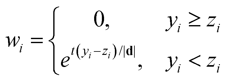
Given m and σ, the logistic function is depicted in Fig. 1. Considering that it is practically 1 when d < 0, i.e., y_i < z_i as you see in the figure, only one logistic function in eqn (10) is enough instead of two terms in eqn (9). We express the weights in that way only to emphasize its asymmetric properties.

Fig. 1 Generalized logistic function of the proposed method.

The logistic function gives nearly the same weight to the signal below or above a baseline when the difference between the signal and the baseline is smaller than the estimated noise mean. It gradually reduces the weight as the level of the signal increases. If a signal is in the 3σ from the estimated noise mean which covers 99.7% of noise on Gaussian assumption, small weight is still given. Finally, zero weight is given when a signal is much higher than the baseline as it can be regarded as a part of the peak. In the extreme case the standard deviation is nearly zero, it becomes a shifted and reversed unit step function which smoothes and estimates a baseline while leaving the peak larger than noise mean untouched.

Modifications of eqn (10) would be possible. As the essence of the proposed method is to give a proper weight to a signal above a baseline as well as a signal below the baseline in the pure baseline region, one could push the curve of the logistic function to the left or to the right direction so long as it gives a meaningful weight to a signal above the baseline. Also squeezing the transient region would be possible. For example, one can narrow the region arbitrarily to get the result of the extreme case.

The smoothed baseline can be obtained by using the same iterative procedure as AsLS and airPLS methods. Assume that the first baseline z is computed with w initialized to have ones. Get a new w according to eqn (9). Then solve eqn (5) again to get an updated baseline z. The iteration continues until weights do not change anymore or weight changes are minimal.

Let y be the measured spectrum expressed as a column vector with N elements. Given the smoothness parameter λ, the proposed arPLS (asymmetrically reweighted penalized least squares) method can be summarized as an algorithm.

Implementation of Matlab is simple, as the following code shows. To implement the arPLS method in other programming languages, one can refer the books about linear equations with the symmetric pentadiagonal matrix.^17,18 As the matrix, W + H, is sparse and symmetric band diagonal, an efficient algorithm can be easily implemented to solve eqn (5).

4. Experiments

Three simulated spectral data and three kinds of experimental Raman spectra were used to evaluate the performance of the proposed method. All the experiments were carried out using the Matlab software package (MathWorks, MA, USA).¹⁹

4.1 Simulated data

Three simulation data were generated using well-known analytic functions. They are intended to imitate real spectral data that contain a varying baseline, analytical signal, and random noise. In Fig. 2, the simulated pure signal is shown which contains three Gaussian peaks that are given as follows:where i = 1, 2, …, 1000. The heights of three peaks are 100, 200, and 113.7 from left to right.

Fig. 2 Simulated spectrum without baseline and noise.

Noise, n, was modeled using a uniform random number generator and a third order polynomial function was used to simulate a curved baseline in a concave and convex region. Narrow Gaussian peaks were treated as the spectra of interest. The simulated spectra were generated by adding a pure signal, a baseline, and random noise.

Two simulated data with a curved baseline are shown in Fig. 3. The SNR (Signal to Noise Ratio) of the low noise spectrum was set to 17.7 dB and that of the high noise spectrum was set to 31.7 dB. The SNR with respect to energy was measured without the baseline according to the following equation:

SNR = 10 log₁₀(E_s/E_n) (12)

Fig. 3 Simulated spectra in high and low noise.

The maximum iteration number was set to 50 for all three methods. For early termination, the termination ratio was set to 10⁻⁶ for AsLS and arPLS while eqn (8) was used for airPLS.

The proposed method, arPLS, was compared with AsLS and airPLS methods. Before the experiments, the smoothness parameter, λ, was tuned to get a good estimation of the baseline. If λ is too large, a fitted baseline would not catch the curved baseline. On the other hand, a fitted baseline would follow peaks if λ is too small.

All three methods would show a little different performance according to various λ. So experiments with various λ were carried out to see the behaviour of the methods and find the optimum λ. As we know the exact spectrum is given as eqn (12) for the simulated spectra, we can compare the performance of three methods using RSME (root mean square error). Assuming that the baseline corrected spectrum is s with given λ, RSME(λ) is defined as

In order to find the optimal value, λ is changed from 10² to 10⁸ as λ is recommended to vary in the log scale.¹⁶ In Tables 1 and 2, we show the RSMEs of the baseline corrected spectra obtained from three methods.

Table 1 RMSE of baseline corrected spectra in low noise

	log10 λ
	2	3	4	5	6	7	8
AsLS	23.4	8.63	3.77	6.25	15.4	21.1	22.1
airPLS	30.4	26.3	5.30	2.92	5.21	17.8	22.4
arPLS	39.5	23.6	1.93	1.22	1.19	2.98	6.01

---

Table 2 RMSE of baseline corrected spectra in high noise

	log10 λ
	2	3	4	5	6	7	8
AsLS	23.9	12.3	11.2	12.6	22.4	27.9	29.0
airPLS	31.7	24.6	10.5	10.9	11.6	24.2	29.7
arPLS	44.5	39.65	23.1	6.10	5.74	5.86	7.24

---

The least RSMEs of each method in low noise are found at λ = 10⁴, 10⁵, and 10⁶ while they are found at λ = 10⁴, 10⁴, and 10⁶ in high noise. They are displayed in Fig. 4 for easy comparison. The RSME of arPLS is about half of the other methods, which means that the baselines are more accurately fitted by arPLS.

Fig. 4 RMSE of baseline corrected spectra with optimal λ.

Let us see the baseline corrected spectra in detail. In Fig. 5 and 6, all the baseline corrected spectra by three methods are shown. As you see in the figures, the baselines are well-estimated and removed by arPLS. Especially in the non-signal region, the other two methods show some biases caused by the underestimated baseline.

Fig. 5 Baseline corrected spectra in low noise.

Fig. 6 Baseline corrected spectra in high noise.

There are also some biases in estimating the height of peaks. In the low noise spectrum, it is observed that airPLS underestimates the height of the second peak more than the others while AsLS and airPLS overestimate the height of the first and the second peaks more than arPLS in the high noise spectrum. That is the effect of additive noise.

In addition to them, there is one thing more to mention. As you see in the tables, the optimal λ is slightly different between the methods. As the parameter should be set manually for practical applications, it would be better if baseline correction performance is not too sensitive to λ.

In Fig. 7, the RSME of arPLS for various λ is displayed. While the lowest RSME is obtained when λ = 10⁵ in the low noise spectrum, similar performance can be obtained when 10⁴ ≤ λ ≤ 10^6.5. Even up to 10⁷, the RSME of arPLS is comparable to the best case of the other methods. In the high noise spectrum, the arPLS method keeps the low RSME when 10^4.2 ≤ λ ≤ 10^8.2. This means that arPLS is relatively robust to the choice of λ, which is desirable for practical applications.

Fig. 7 RMSE of arPLS for various λ.

Another set of experiments was carried out with a simulated spectrum with a linear baseline. As linear baseline correction is rather simple, a spectrum with a strong baseline in high noise is only considered here. The simulated spectrum is shown in Fig. 8. Baseline corrected spectra obtained using AsLS, airPLS, and arPSL are given in Fig. 9. The processing results are very similar to those shown in Fig. 6. There are some bias in the non-signal region and the height of peaks is overestimated by AsLS and airPLS. The measured RSME of arPLS was 6.1 while those were 10.9, 10.5 for AsLS, airPLS, respectively.

Fig. 8 Simulated spectrum with linear baseline.

Fig. 9 Baseline corrected spectra with linear baseline.

These consistent results confirm that arPLS has the better capabilities in eliminating a baseline in the non-signal region and estimating the height of peaks. So we hope that the arPLS could be a promising alternative to the existing methods.

4.2 Experimental Raman spectrum

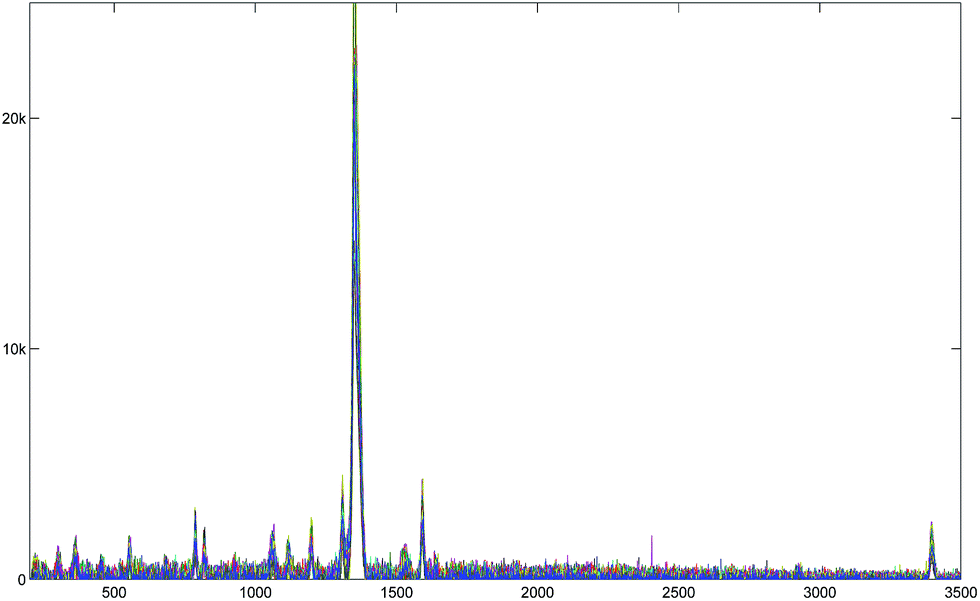
The Raman spectra of three materials were used for the experiments. They are 26DNT (2,6-dinitrotolune), 35DNT (3,5-dinitrotolune), and 2ADNT (2-amino-4,6-dinitrotolune). In recording Raman spectra, the laser power was kept lower than 1.0 mW to avoid laser heating.²⁰ The Rayleigh line was removed from the collected Raman scattering using a holographic notch filter located in the collection path. Spectra were collected via a static scan in the region of 200–3500 cm⁻¹. The collection time was 5 seconds and a 50× objective lens was used to focus the laser.

A single 26DNT spectrum was tested and is shown in Fig. 10 together with the baseline corrected spectra. All the three methods were used to obtain baseline corrected spectra. The figure shows that AsLS and airPLS methods underestimate the baseline especially in right half of the non-signal region, which is also observed with the simulated spectra. This might lead to overestimation of the height of peaks in the region. But we cannot confirm that as the exact heights of those peaks are not given for the experimental Raman spectrum.

Fig. 10 Baseline corrected 26DNT Raman spectra.

The other two kinds of spectra were processed to show the capability of the proposed method. They are measured in highly fluorescent baselines. The 35DNT is chosen as an example of a spectrum with linear background in low noise while 2ADNT is chosen as an example of a spectrum with highly curved background in high noise. Two sets of 50 spectra are shown in Fig. 11 and 13. Even though they were measured by the same spectroscopy, they showed varying baselines according to the samples in issue.

Fig. 11 Measured 35DNT Raman spectra.

Fig. 12 Baseline corrected 35DNT Raman spectra.

Fig. 13 Measured 2ADNT Raman spectra.

The baseline corrected spectra obtained using the arPLS method are shown overlapped in Fig. 12 and 14. As you see in the figures, all the baseline corrected spectra from the same material looks quite similar, which is natural and desirable. So we could say that all the baselines of two sets are successfully removed by our method and then they can be analyzed easily.

Fig. 14 Baseline corrected 2ADNT Raman spectra.

Finally, it is worth noting that the smoothness parameter λ is set to 10⁵ throughout the experiments with the experimental Raman spectra for the arPLS method. As the baseline corrected spectra are acceptable as you see in the figures with the value obtained from simulation data, we could convince that arPLS is robust to the variation of λ as mentioned previously.

5. Conclusions

The proposed arPLS method provides a simple but effective algorithm for estimating baselines in analytical chemistry. It gives fast and accurate baseline corrected signals for both simulated and real spectra. The experimental results with the simulated spectra confirm that the arPLS method yields better results than AsLS and airPLS methods in baseline correction and peak height estimation. Experiments with Raman spectra also show that the arPLS method could handle various kinds of baselines in real spectra.

We are currently investigating the method to adjust the smoothness parameter automatically. Except for it, the arPLS method requires no prior knowledge about the sample composition, no peak detection, and no mathematical assumption of background noise distribution. So it could be easily applied to various spectra. We hope that the proposed method would be a promising alternative to the existing baseline correction methods and widely used by many researchers.

Acknowledgements

This research was supported by the Basic Science Research Program through the National Research Foundation of Korea (NRF) funded by the Ministry of Education (2013K2A2A).

References

1. H.-W. Tan, C. R. Mittermayr and S. D. Brown, Appl. Spectrosc., 2001, 55, 827–833.
2. H.-W. Tan and S. D. Brown, J. Chemom., 2002, 16, 228–240.
3. P. J. Gemperline, J. H. Cho and B. Archer, J. Chemom., 1999, 13, 153–164.
4. A. Likar and T. Vidmar, J. Phys. D: Appl. Phys., 2003, 36, 1903–1909.
5. Y. Hu, T. Jiang, A. Shen, W. Li, X. Wang and J. Hu, Chemom. Intell. Lab. Syst., 2007, 85, 94–101.
6. J. C. Cobas, M. A. Bernstein, M. Martin-Paster and P. G. Tahoces, J. Magn. Reson., 2006, 135, 1138–1146.
7. Z.-M. Zhang, S. Chen and Y.-Z. Liang, Talanta, 2011, 83, 1108–1117.
8. S.-J. Baek, A. Park, J. Kim, A. Shen and J. Hu, Chemom. Intell. Lab. Syst., 2009, 98, 24–30.
9. T. Vickers, R. Wambles and C. Mann, Appl. Spectrosc., 2001, 55, 389–393.
10. V. Mazet, C. Carteret, D. Brie, J. Idier and B. Humbert, Chemom. Intell. Lab. Syst., 2005, 76, 121–133.
11. F. Gan, G. Ruan and J. Mo, Chemom. Intell. Lab. Syst., 2006, 82, 59–65.
12. S.-J. Baek, A. Park, A. Shen and J. Hu, J. Raman Spectrosc., 2011, 42, 1987–1993.
13. S. Wartewig, IR and Raman Spectroscopy, WILEY-VCH, Germany, 2003.
14. P. H. C. Eilers and H. F. M. Boelens, http://www.science.uva.nl/%7Ehboelens/publications/draftpub/Eilers_2005.pdf, 2005.
15. Z.-M. Zhang, S. Chen and Y.-Z. Liang, Analyst, 2009, 135, 1138–1146.
16. P. H. C. Eilers, Anal. Chem., 2003, 75, 3631–3636.
17. W. H. Press, S. A. Teukolsky, W. T. Vetterling and B. P. Flannery, Numerical Recipes in C, Cambridge University Press, 1992.
18. J. Kiusalaas, Numerical methods in Engineering with Matlab, Cambridge University Press, 2005.
19. The MathWorks, Statistics Toolbox User's Guide, The MathWorks, Inc, USA, 2014.
20. J. Hwang, N. Choi and A. Park, et al. , J. Mol. Struct., 2005, 1039, 130–136.

---