A signal deconvolution method to discriminate smaller nanoparticles in single particle ICP-MS
Geert
Cornelis
* and
Martin
Hassellöv
University of Gothenburg, Chemistry and Molecular Biology, Kemivägen 10, Göteborg, Sweden
First published on 2nd October 2013
Abstract
Single particle ICP-MS (spICP-MS) analysis of inorganic nanoparticles (NPs) cannot accurately distinguish dissolved ion signals and signals from relatively small NPs, although these particles are often more reactive than their larger counterparts. A signal deconvolution method was developed for spICP-MS analysis using gold (Au) NPs of nominally 10, 15 or 30 nm diameter. The signal distributions of dissolved Au standards were parameterised as a function of concentration using a mixed Polyagaussian probability mass function. Dissolved curves were fitted using this parameterisation to the low-intensity signals of samples containing NPs to subtract and deconvolute the dissolved signals from the particle signals. The dissolved signals were quantified in this process. The accuracy of the deconvolution method was confirmed for all NP suspensions studied when comparing the size and number concentration obtained with the deconvolution method with values based on transmission electron microscopy. This method thus allows analysis of NP suspensions with spICP-MS where it was hitherto not possible. The applicability domain lies predominantly with relatively small NPs and/or when a relatively high concentration of dissolved ions of the element of interest is present, where overlapping between dissolved and particulate signals occurs.
Introduction
The need for sensitive techniques to quantify both size and particle number concentration of nanoparticles (NPs) in aqueous samples has to a great extent been driven by research on the fate and effects of engineered nanoparticles (ENPs) in the environment. There are indications that ENPs are potentially harmful to organisms, but the effects depend highly on the concentration, size and in which form the nanoparticles are presented to organisms.1 It is therefore crucial that ENP exposure is assessed in situ to have a realistic assessment of risk. However, in situ ENP characterization is challenging, owing to the likely low environmental concentration (<106 particles per mL; <ng L−1), the high abundance of natural NPs, and the presence of interfering elements.2 Analysis of such samples is not possible with currently available techniques. Electron microscopy methods, for instance, have been shown to provide powerful information,2 but sample preparation artefacts, the high particle count required and unsuitability for high-throughput applications limit the applicability of these techniques for assessment of ENP size and particle number in environmental samples.Single particle inductively coupled plasma-mass spectrometry (spICP-MS) is a promising technique to quantify the particle number size distribution (PSD) of metal containing NPs in liquid samples at low total particle number concentrations.3–6 If a sufficiently dilute suspension of inorganic particles is nebulized into the plasma, then a burst of ions will be generated when each discrete particle is vaporized, atomized and ionized. When these ions arrive at the detector, an intense output signal is generated of which the intensity is related to the mass of the particle and therefore its size, if a spherical shape is assumed. The particle number concentration is related to the detected particle burst frequency. The PSD can in principle thus be calculated. Moreover, the fast measurement frequency of spICP-MS allows counting statistically significant particle numbers from relatively dilute NP suspensions in a short time and the element-specificity of ICP-MS allows discerning ENPs from naturally occurring NPs having a different elemental composition.3
The spICP-MS technique has in recent years been further developed. A wide range of NP materials with smaller diameters has been analysed, distinction between simultaneously occurring NP signals and signals from dissolved ions of the mass of interest has been investigated and spICP-MS has been applied to environmental samples.3,5–10 However, some important limitations still remain. spICP-MS can in theory be used to measure particle sizes of 10 nm or lower.3,6 There is, however, no accurate method by which NP signals can be distinguished from the continuous background signal of dissolved analytes. The mean intensity of the continuous signal can be high, e.g. if an element with a relatively high natural background is measured, or it can be relatively low, but there is always a non-zero continuous background signal.
Analysing small NPs selectively with spICP-MS may be beneficial, given that the reactivity and possibly also toxicity of NPs often increase with decreasing particle size,1 but the lowest NP size that spICP-MS can accurately detect is limited in the presence of background signals that are highly relative to the particle signals. Particularly if the particles are composed of elements to which ICP-MS is less sensitive such as Ti, only a small fraction of the atoms in the particle are ionised in the plasma and arrive at the detector. The dissolved background may be lower when measuring diluted samples, but dilution may be undesirable when analysing extremely low particle number concentrations, a situation that poses challenges for the spICP-MS analysis of particles composed of e.g. ZnO that may occur together with relatively high natural background concentrations of dissolved Zn.
Discerning particle signals from dissolved signals is currently often not done by an objective method. Lower intensity signals are simply regarded as emanating from dissolved ions and higher intensity ones are regarded as being particulate. Attempts towards a more objective method to distinguish particle signals use threshold limits of a number of times the standard deviation of the continuous signal and particle signals are identified as the outliers relative to this threshold value.3 A mean dissolved intensity is subsequently subtracted from all particulate signals. Both approaches work well if the signals of all particle ion bursts are clearly outliers from the continuous signal.5 When the particle signal intensities are much smaller compared to the continuous background signal, PSD determination becomes inaccurate, because a significant fraction of the particle signals may be recognized as dissolved signals or vice versa by the subjectively set threshold limit.3
The present paper presents an objective, mechanistically based method where dissolved signals are deconvoluted from particulate signals, because such a method could allow distinction of smaller particles from the background than hitherto possible.
Theory
Overview
Fig. 1 shows a schematic overview of the proposed deconvolution method. Considering ICP-MS signals not in time space but in intensity–space, i.e. as frequency–intensity histograms, is crucial to this method. This approach is not fully new to spICP-MS data treatment. In fact, after removing signals that are considered emanating from dissolved ions, signal histograms of spICP-MS measurements are used to calculate the sought-after PSD.11 New in the proposed method is regarding also the blanks and soluble standards in intensity-space during the calibration stage allowing statistical analysis of these signals (Fig. 1a). Polyagaussian (PG) probability mass functions (pmfs) are fitted to relative frequencies (i.e. frequencies divided by the total number of measurements of D). A set of pmf parameters is thus obtained for each blank or standard. There are theoretical relationships between these parameters and with the analyte concentrations that can be studied using linear regression analysis. Using these relationships, the pmf of dissolved signals can be accurately reconstructed using only a limited number of relative frequencies. | ||
| Fig. 1 Overview of the convolution method showing the different steps of the (a) calibration stage using blanks and dissolved standards and (b) data-analysis of spICP-MS measurements of particle suspensions. The cross-cutting arrows show in which stages of spICP-MS data analysis that information obtained during the calibration stage is used. Symbols are explained in the list of symbols and throughout the text. | ||
spICP-MS data are collected using the same measurement conditions (i.e. D, dwell time, sensitivity, …) as for blanks and dissolved standards (Fig. 1b). There is an unknown number Dd of all measurements of D in these spICP-MS data where no particle ions arrived at the detector. It is known that these measurements have a lower mean intensity than those measurements during which particle ions arrived at the detector. It is also known that particle-free measurements have the same signal distribution as dissolved ions and can thus be described using the same pmfs fitted during the calibration stage. A Polyagaussian pmf is therefore fitted to the relative frequencies of the lowest intensities of spICP-MS data. The relative frequencies need, however, to be calculated using the unknown number Dd which is therefore varied along with the parameters of the pmf during the fitting stage until the sum of squares error is minimal. The fitted pmf is then multiplied with Dd to obtain a histogram of actual frequencies of dissolved signals. This histogram is then subtracted from the spICP-MS histogram, leaving a histogram representing the distribution of Dp = D − Dd measurements during which a particle arrived at the detector. These measurements still contain a dissolved component, because dissolved ions arrived together with particles at the detector. The fitting operation provided exact knowledge on the pmf of the dissolved signal, which can therefore be deconvoluted from relative frequencies of the combined signal (calculated by dividing frequencies with Dp). The deconvoluted relative frequencies are then multiplied with Dp to obtain a histogram of actual frequencies of filtered particulate signals. This histogram can be recalculated into a PSD using known spICP-MS theory.
Signal distributions of dissolved signals
An ICP-MS measurement Id of a dissolved analyte sample with concentration C in pulse counting mode is the number of ions, hereafter called counts, arriving at the electron multiplier during the dwell time td. Repeated measurements of Id vary as a function of time because of noise. Noise of ICP-MS signals has two main components.12Shot noise is caused by random arrival of ions at the detector during td. Flicker noise is caused by physical processes during sample introduction such as fluctuations in arrival times of droplets in the plasma, fluctuations in ion travel speeds through the mass spectrometer, ion diffusion in the plasma and mass spectrometer, and fluctuating ionization because of differently sized nebulized droplets being introduced in the plasma. Dark noise is caused by the electronics of detection, but can in most cases be ignored relative to the previous two independent noise sources.12,13The probability of measuring a particular value of Id in a series of D repeated measurements of a dissolved analyte can be estimated by the relative frequency, i.e. f(Id) × D−1. Such relative frequencies obey some underlying pmf. In discussions pertaining to e.g. detection limits of ICP-MS, it is mostly assumed that the relative frequencies of low-intensity signals follow a Poisson distribution assuming perfectly random arrival of ions at the detector12 whereas at higher counts, it has been suggested that the distribution of dissolved signals can be described with a Gaussian distribution.6 The present method requires a pmf that describes the signal distribution of all signals, regardless of the average signal intensity. ICP-MS signals are therefore seen as a sum of two random variables S and F to represent those components of Id that are distorted differently by respectively shot and flicker noise.
| Id = S + F | (1) |
The standard deviation of the shot noise component, σs, is often also called the shot noise amplitude. With λ the mean intensity, the shot noise variance σs2 equals λ in the case of Poisson statistics. However, there are many processes that make signals from electron multiplier detection overdispersed with respect to a Poisson distribution, i.e. σs2 > λ.13–15 In such cases, the Polya pmf is often used14,16
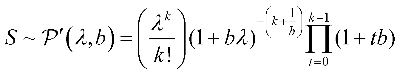 | (2) |
Eqn (2) shows that the Polya pmf has in addition to λ a parameter b, the shape factor. The Polya pmf is in fact a family of pmfs that includes for instance the Poisson distribution for b → 0. The less common notation of Prescott16 is used in eqn (2) where the parameter λ is also the mean measured signal making it more convenient to compare the Polya to the Poisson pmf. Relations with more common notations can be found in the appendix.
The intensity distribution of ICP-MS signals of higher counts where flicker noise dominates is usually described relatively well using a Gaussian pmf N(μf,σf) having the mean, μf, and standard deviation, σf, as parameters.12 It follows from statistical theory and eqn (1) that μf = 0 because if expected values are calculated, eqn (1) becomes E(Id) = E(S) + E(F) while E(F) equals μf and both E(Id) and E(S) equal λ. The standard deviation of the flicker noise component, σf, is often called the flicker noise amplitude. The discrete approximation of the continuous Gaussian probability density function based on Kemp17 as parameterised by Harris et al.18 was used in this work. The pmf of flicker noise is thus described by F ∼ N(0,σf).
The pmf of a sum of two independent random variables is the convolution of the individual pmfs of those variables. The pmf for Id is thus a compound, also called a mixed, distribution of the Polya pmf for the shot noise component on the one hand and a Gaussian pmf for the flicker noise on the other hand. Such compound distributions are hereafter called Polyagaussian pmfs.
Calibration of the deconvolution method
In the proposed method, Polyagaussian pmfs are fitted to ICP-MS signal distributions of several blanks and dissolved standards with a known concentration C, blanks having C = 0. The fitting procedure, minimization of the negative log(likelihood), is explained in the appendix. This procedure generates estimates of the parameters λ, σ and b for each blank or dissolved standard. The interrelation between these parameters and the relation with the concentration of the dissolved standards can then be studied further.λ is linearly related to C according to eqn (3), which is a classical ICP-MS calibration curve:
| λ = mC + Ibkg | (3) |
 | (4) |
In the literature on photomultiplier detectors that behave similarly to electron multipliers in terms of shot noise,14 the shot noise component is calculated as
| σs2 = βλ | (5) |
 | (6) |
At higher mean intensities, flicker noise dominates the total noise amplitude. It is well known that the flicker noise amplitude σf increases linearly with the mean signal intensity λ:12,13,19
| σf = ξλ | (7) |
Fitting the dissolved signal to mixed signals
A nanoparticle suspension will always produce a combined signal Ip, one that is caused partly by dissolved ions and partly by particles. eqn (1) needs to be rewritten for such signals as:| Ip = Id + P = S + F + P | (8) |
When the best fit of the dissolved signal is found, the number of particle events is found as well because
| D = Dd + Dp | (9) |
D p is the number of measurements that contain particle signals. In addition, the dissolved concentration can be calculated using eqn (3), provided that this concentration is above the detection limit.
Deconvolution of the dissolved signal from mixed signals
The histogram of the dissolved analytes can be calculated from the fitted Polyagaussian pmf by multiplying it with Dd. This histogram is then subtracted from the histogram of the total signal, a procedure that effectively removes the frequencies of Dd measurements containing only dissolved signals. The resulting histogram represents Dp measurements that obey eqn (8) with P > 0 for each measurement. The histogram therefore still contains a dissolved component (S + F). The corresponding relative frequencies of this histogram, Ct = f(Ip) × Dp−1, have an underlying pmf that is a convolution of the pmf of dissolved signals (PG) and an underlying pmf of the particulate signals (Cp), because the pmf of the sum of two variables is the convolution of the individual pmfs.| Ct = PG × Cp | (10) |
The pmf of the dissolved signal (PG) is known as it has been fitted during the previous step. This pmf can thus be (numerically) deconvoluted from Ct to obtain at least an estimate of the pmf of particle signals, Cp, devoid of noise components caused by the dissolved signal. It follows from eqn (8) that E(P) = E(Ip) − E(S + F) and Var(P) = Var(Ip) − Var(S + F) or in other words, deconvolution is expected to reduce the mean signal as well as the broadness of the histogram.
The deconvolution procedure of Matlab (Version 7) was used in the present study, which did not always succeed to produce meaningful results for all particle suspensions. In those cases, further calculation was done using Ct instead of Cp because it will be argued that in most cases, Var(S + F) is much smaller than Var(Ip), i.e. the contribution of PG is relatively small so that Ct is actually a good estimate of Cp.
Particle size distributions
The histogram Cp × Dp (or Ct × Dp) holds the actual frequencies of particle signals P and can be calculated into a PSD, mostly using the established spICP-MS theory.11 This theory uses the mean intensity–concentration calibration (eqn (3)) to calculate the relation between measured intensity of each particle event and mass per measurement event W: | (11) |
η neb is the dimensionless nebulization efficiency, i.e. the fraction of the analyte that passes through the nebulizer and spray chamber into the plasma, qliq is the flow rate of sample into the nebulizer, and td is the dwell time. m is the sensitivity and Ibkg is the average signal intensity in blank samples, both determined during calibration (eqn (3)). The mass is then calculated into diameter di, assuming a spherical size:
 | (12) |
η i is the ionization efficiency, which is assumed to be 1. fa is the molar fraction of the element that is measured in the particle and ρ is the particle density (kg m−3). Eqn (12) was taken from Pace et al.11 whose method required an assessment of Id, the mean dissolved concentration. Id = 0 in the case Cp is used to calculate the PSD because the dissolved signal is removed from the data during the deconvolution stage. The actual particle number concentration of each size can be obtained using eqn (13).
 | (13) |
The total particle number concentration nt can be calculated by replacing f(Pi) by Dp.
Experimental section
Chemicals
Dissolved Au standards were prepared from a 1000 mg L−1 Au standard in 5% (v/v) hydrochloric acid (HCl). NP suspensions were prepared from citrate coated gold nanoparticle suspensions having nominal diameters of 10, 30 or 60 nm (NIST, USA) or 15 nm (BBI, UK).Nanoparticle characterization
There are currently no reference methods to directly measure particle number concentrations in ENP suspensions. The number concentrations were therefore estimated from total Au mass concentrations combined with PSDs determined using TEM analysis. The total Au mass concentration was determined after a microwave (Milestone) digestion of 5 mL of the suspension in aqua regia at 180 °C (maximum power 1000 W). The PSD of 15 nm NPs was determined using transmission electron microscopy (TEM). A drop of suspensions was air-dried on a 15 mesh carbon coated copper grid and particle sizes were measured and counted using ImageJ software (US National Institute of Health). TEM data for the 10 and 30 nm NPs were taken from NIST documentation.AuNP spICP-MS measurements
A sector-field ICP-MS (Thermo Element 2 settings given in Table 1) was used in all experiments. The nebuliser gas flow rate and sample delivery rate (Table 2) were optimised to maximize both sensitivity and short-term stability using 1 μg L−1 115In in 2% nitric acid (HNO3). All dissolved Au standards and AuNP suspensions were diluted using a 0.1% cysteine solution to reduce memory effects.20| ICP-MS | Thermo element 2 |
|---|---|
| Spray chamber | Glass expansion 4 mL Twinnabar (cyclonic) |
| Nebuliser | Glass expansion ca. 400 μL min−1 Micromist (conical) |
| Cool gas flow rate | 15 L min−1 |
| Auxilliary gas flow rate | 0.96 L min−1 |
| RF Power | 1240 W |
| Mass resolution | Low |
| a Error boundaries indicate standard deviation on three repeated measurements. b Error boundaries indicate number based standard deviation of the diameter. | |||||
|---|---|---|---|---|---|
| Nominal NP size (nm) | 10 | 15 | 30 | ||
| Au mass concentration (mg L−1) | 58 ± 2a | 71 ± 1 | 62 ± 3a | ||
| Mode diameter (TEM) | 9 ± 1b | 15.0 ± 0.2b | 28 ± 2b | ||
| Total particle number concentration (based on TEM and total mass concentration) N (mL−1) | 8.44 × 10¹² | 6.01 × 10¹¹ | 2.14 × 10¹¹ | ||
| Number of datapoints (D) | 10![[thin space (1/6-em)]](https://www.rsc.org/images/entities/char_2009.gif) 000 000 |
10000 |
10000 |
||
| Dwell time td (ms) | 1 | 1 | 5 | 1 | 5 |
| Nebuliser gas flow rate (L min−1) | 1.12 | 1.12 | 1.11 | 1.11 | 1.11 |
| Nebulisation efficiency ηn (%) | 12 ± 2 | 10 ± 1 | 12 ± 1 | 10.5 ± 0.4 | 10.5 ± 0.3 |
| Sample flow rate qliq (μL min−1) | 448 ± 4 | 425 ± 3 | 425 ± 4 | 432 ± 4 | 433 ± 3 |
| Sensitivity m (count L ng−1) | 0.90 | 1.04 | 4.47 | 0.90 | 3.83 |
| Blank counts Ibl (counts) | 17.5 | 11.7 | 19.6 | 1.5 | 19.4 |
| Flicker coefficient ξ | 0.06 | 0.11 | 0.10 | 0.25 | 0.25 |
| Shot coefficient β | 1.73 | 1.68 | 2.0 | 3.18 | 1.98 |
Dissolved standards of 1, 5, 10, 30, 100, 1000 and 2000 ng L−1 were thus prepared while NP stock suspensions were diluted up to 108 times. Each measurement batch consisted of five blanks of 0.1% cysteine, dissolved standards, a 106 times diluted 60 nm Au NP suspension for nebulisation efficiency determination (see further), a dilution series of one NP suspension of one size (10, 15 or 30 nm) and finally again a 60 nm Au NP suspension. Each measurement batch was measured at a nominal dwell time of 1 or 5 ms during ICP-MS measurements, and 10000 measurements were collected in counting mode. Between each sample measurement the probe was rinsed using 2% HNO3. Calibration curves, frequency histograms and particle counts were calculated from the exported raw data using the above spICP-MS theory that was programmed in MATLAB (version 7).
Nebulisation efficiency determination
The method of Pace et al.11 was used to determine ηneb during each measurement batch. This method calculates ηneb using the certified size or the particle number concentration of 60 nm NIST Au NPs and eqn (12) or (13), respectively. Flow rates during measurement were measured with a Truflow flow meter (Element Scientific, USA). The spICP-MS data of 60 nm NP samples were deconvoluted similarly to other samples, a procedure that results in the knowledge of Id for these samples. This value and the certified size of the NIST 60 nm Au NP standard could then be used to calculate ηneb according to eqn (12).Results and discussion
Nanoparticle characterization
Table 2 lists the main properties of the NP suspensions used in this study. The PSDs calculated from TEM analysis provide a set of relative particle number concentrations (n1,…,nk) of discrete bins of average diameters (d1,…,dk). Those number concentrations nk are related linearly to nt by a constant K that can be estimated by assuming a spherical shape for the particles and relating K to the total mass concentration C (g L−1) that was measured after digestion: | (14) |
Noise distribution of dissolved ICP-MS signals
Fig. 2 shows Polyagaussian pmf fits to the relative frequencies of the signals of one blank and two dissolved standards. It can be seen that the fits are satisfactory regardless of the average intensity λ and the dwell times used (1 or 5 ms). | ||
| Fig. 2 Signal distributions, Polyagaussian and Poissongaussian pmf fits of dissolved ICP-MS signals of a blank or a 30 ng L−1 dissolved standard acquired at 1 or 5 ms when measuring 15 nm Au NPs. The Polyagaussian and Poissongaussian pmfs overlap in the case of the 30 ng L−1standards. | ||
While a wealth of literature can be found on origins of noise in ICP-MS signals (e.g.ref. 12, 21 and 22), the most appropriate pmf describing the signal noise distribution has rarely been investigated. The Poisson pmf was the most appropriate distribution in the study of Laborda et al.6 who also suggested that this pmf is appropriate for signal distributions of dissolved silver ions, at least up to 30 counts. It was therefore attempted also to fit the relative frequencies of blanks and dissolved standards with a mixed Poissongaussian pmf. The difference with the Polyagaussian pmf is that the shot noise component of eqn (1) is modelled using a Poisson pmf instead of a Polya pmf. Shot noise dominates at low mean signal intensity λ, e.g. in the case of blank signals. It can thus be expected that these signals should be predominantly Polya or Poisson distributed. The standard deviations of all blanks in this study were overdispersed with respect to the mean value, i.e. σt2 > λ, which implies that a Poisson pmf is not appropriate to model shot noise, whereas a Polya pmf appeared to be more appropriate.
At a relatively high λ, flicker noise dominates. The shot noise component S, modelled by a Poisson or Polya pmf, has only a minor contribution to the overall pmf in this case. The dissolved pmf in this case is predominantly Gaussian. The Polyagaussian pmf appears to be an appropriate pmf to model the signal distribution of ICP-MS signals of dissolved analytes, regardless of the mean signal intensity. This pmf can therefore be used in the proposed deconvolution method, both in the case where the dissolved signal has a low mean intensity and when the signal intensity is higher, i.e. when a measurable dissolved analyte concentration is present.
Calibration
Fig. 3 shows that the linear relations predicted by eqn (3), (6) and (7) are valid, regardless of the dwell time used. The values for calibration parameters obtained in all measurement runs are shown in Table 2. | ||
| Fig. 3 Calibration of spICP-MS deconvolution for the measurement batch of 15 mn Au NPs measured at 5 ms dwell time. The linear fits and Pearson correlation coefficients: (a) dissolved standard Au concentration vs. λ (eqn (3)). (b) λ vs. σ (eqn (7)). (c) log(λ) vs. log(b) (eqn (6)). Fig. 3d shows log(σt) vs. log λ and the predicted trend according to eqn (15). | ||
From eqn (1) it follows that the total variance σt2 = σs2 + σf2. Combining this equation with eqn (4) and (5) results in
 | (15) |
Fig. 3d shows that eqn (15) fits experimental data really well, again demonstrating the validity of eqn (4)–(8) that can therefore be used in combination with the Polya pmf to model the noise distribution of dissolved signals in the next step of the deconvolution method.
While the linear relations between mean intensity (λ) and concentration or flicker noise amplitude have been studied extensively, the dependency of the form factor (b) of the Polyagaussian on λ as mediated by the shot noise coefficient has not. The shot noise coefficient is only mentioned in the literature on inductively coupled plasma atomic emission spectrometry using photomultiplier detectors13 but not in noise analysis studies of ICP-MS where it is mostly assumed that noise should behave Poissonian (e.g.ref. 12). However, early work by Prescott et al.16 revealed that the Polya model is more appropriate to describe the counting statistics for photomultiplier tubes, whereas Dietz et al.14,23 showed that the same pmf applies in the case of the counting statistics of electron multiplier detectors. Stochastic processes occurring in the electron multiplier have been suggested to explain this overdispersion, i.e. σt2 > λ, of the counting signals with respect to the Poisson pmf.14,24 On the other hand, the Polya pmf is often used to model occurrences of rare events that do not occur entirely random, but that are to some degree correlated, such as the geographic occurrence of earthquakes.25 It has recently been suggested that ions exhibit some degree of attraction in plasmas despite being of the same charge.26 Such processes may lead to some degree of clustering of ions in plasmas and thus ions possibly do not arrive perfectly randomly at the detector.
Table 2 shows the nebulisation efficiencies, sensitivity, shot and flicker factors for all measurement batches. The number of measurement batches and the variation in obtained values were probably too limited to observe correlations between these parameters. Moreover, the relation between these parameters is most likely complex, involving more parameters than those determined in this study.
Overlap between dissolved and particulate signals
It will be argued that the deconvolution method is most useful to analyse spICP-MS signals where the dissolved peak overlaps with the particle signal. This occurs when the particles are relatively small and/or when the dissolved signal intensity is relatively high. Using lower dwell times may also increase overlap. Using lower dwell times lowers the dissolved signal intensity, but the proportion of incompletely measured particle events increases thus broadening the particle signal distribution to lower signal intensities.3Fig. 4 shows the histograms of spICP-MS data acquired at different dwell times. Particle suspensions with monomodally distributed particle sizes always show two peaks, one for the dissolved signals and one for the particle signal. This is most clearly visible in the case of 15 nm Au NPs measured at 5 ms in Fig. 4. In the case of dilute suspensions, the majority of the signals does not contain a particle event. The frequency of dissolved signals is therefore usually higher than the frequency of particle events. Fig. 5 shows examples where this is not the case. As the particle number concentration increases, the frequency of dissolved signals decreases (Fig. 5a) until there is no dissolved peak left (Fig. 5b). In the latter case, the average signal has increased to 1000 ion counts, because on average twenty particles arrived simultaneously in each dwell and no dissolved model could be fitted to the data.
 | ||
| Fig. 4 The different steps of deconvolution (see Fig. 1) of 10 nm (1.53 × 10⁶ mL−1), 15 nm (9.27 × 10⁴ mL−1) and 30 nm (6.41 × 10⁴ mL−1) Au NPs. The histograms of acquired spICP-MS data are dots, whereas the fitted dissolved curves are shown in blue. The green curves are the frequencies of raw data from which the frequencies of the dissolved fit were subtracted. spICP-MS signals. The insets show more clearly the frequencies of particle signals. | ||
 | ||
| Fig. 5 Histograms and fitted dissolved curves of differently concentrated NP suspensions (a) 6.96 × 10⁵ mL−1 of 15 nm and (b) 5.80 × 10⁶ mL−1 of 15 nm Au NPs measured at 5 ms. (a) The fit of a dissolved curve at which signal intensities single (1), double (2), triple (3) and quadruple (4) particle events occurred. (c) Histograms of 6.41 ×10⁴ mL−1 (full dots) and 3.20 × 10⁴ mL−1 (open circles) of 30 nm Au NPs collected at 5 ms. The fitted dissolved curves are shown in full lines. | ||
Fig. 4 shows that the overlap between dissolved and particulate signal distributions increased with decreasing size. There is some separation in the case of 15 and 30 nm NPs, but the overlap is complete in the case of 10 nm NPs measured at 1 ms, where the particle mass that effectively reaches the detector during a particle event is comparable to the standard deviation of the dissolved signal. The overlap also increases with decreasing dwell time, because the chance of detecting particle events incompletely increases when the dwell time decreases.3,6 Finally, overlap also increases if the concentration of dissolved ions increases, because the standard deviation of the dissolved signal increases too. Fig. 5c compares two spICP-MS measurements of 30 nm Au NP suspensions. The dissolved ion concentration in the least concentrated particle suspension was relatively high, 21 ng L−1, possibly because of contamination or carry-over. The dissolved ion concentration in the more concentrated particle suspensions was only 1.6 ng L−1. The histograms were drawn with different intensity axes so that the average dissolved intensities of both particle suspensions coincided and it can be better observed how much the variation in dissolved signals (S + F) overlaps with the particle (P) signal distribution. A higher dissolved concentration can also increase overlap between particulate and dissolved signals.
Fitting of dissolved signals to combined signals
Fig. 4 shows the dissolved signal frequencies that were fitted to spICP-MS histograms. These are actual frequencies calculated with the fitted Polyagaussian pmf and the fitted value of Dp. More than the theoretical minimum of 2 relative frequencies were needed to accurately fit Polyagaussian pmfs and Dd to spICP-MS histograms.Fig. 6 shows the effect of the number of fit points used to fit Dp for spICP-MS signals of suspensions of 10 nm Au NPs and 15 nm Au NPs measured at 1 and 5 ms, respectively. It can be observed that the fitted Dp remains relatively constant when the fit points are increased above a certain number, indicating that a minimum number of fit points has been reached that leads to an accurate fit. Using less fit points than this minimum number increases the number of false positives (calculated Dp higher than the real value) or false negatives (calculated Dp higher than the real value).
 | ||
| Fig. 6 The number of calculated particle events as a function of the number of fit points used to fit a dissolved curve shown for 10 nm NPs measured at 1 ms (1.53 × 10⁶ mL−1) and 15 nm NPs measured at 5 ms (9.27 × 10⁴ mL−1). Dashed lines indicate the optimum number of fit points. | ||
The requirement of a minimum number of fit points may limit the size of particles that can accurately be deconvoluted from dissolved signals, because the proposed method assumes that the signal intensities used to fit dissolved curves do not emanate from particles. For instance, having to use 6 fit points in the case of the 10 nm Au NPs limits the minimum size of particles that can be accurately distinguished to ca. 6 nm. This limit also depends on the average signal intensity of dissolved ions in the sample. Fig. 6 shows that the minimum number of fit points is higher in the 15 nm NP suspension where the average intensity of the dissolved signal is also higher compared to the 10 nm NPs (Fig. 4).
Deconvolution
Fig. 7 shows the effect of deconvolution of Cp from Ct. The mathematical deconvolution algorithm itself was not refined in this study. The used algorithm only produced meaningful results in those cases when the average dissolved signal intensity was lower than 1, a situation that occurred only in the case of 10 nm suspensions measured at 1 ms. Fig. 7 shows that the deconvoluted signal has a lower mean intensity and standard deviation relative to the combined signal. The decrease in standard deviation was ca. 1% in Fig. 7. Even though deconvolution was not possible in most cases, the standard deviation of Cp could still be predicted because according to the convolution theorem, σ(P) = [σ(Ip)2 − σ(S + F)2]1/2. It was thus estimated that deconvolution would result in 1% or less reduction of the standard deviation of Ct, but deconvolution may have a larger effect if a relatively high dissolved ion concentration would be present in the particle suspension. | ||
| Fig. 7 Effect of deconvolution on the particle histogram and calculated PSD of 10 nm Au NPs (1.53 × 10⁶ mL−1) measured at 1 ms and calculated PSDs of 15 nm (9.27 × 10⁴ mL−1) and 30 nm (6.41 × 10⁴ mL−1) Au NPs measured at 1 or 5 ms, compared to the PSD based on TEM analysis. All PSDs were normalised with respect to the maximum number concentration. The mean values of Ct and Cp are indicated. | ||
Particle size distributions
Fig. 8 shows that the mean diameters according to TEM were accurately reproduced, except in the case of 30 nm Au NPs measured at 5 ms dwell time. Even in the case of 10 nm Au NPs, where overlap with the dissolved signal was significant, the expected mean diameter was reproduced accurately. | ||
| Fig. 8 log(measured/expected) number concentration expressed as particles per mL, as a function of log(expected concentration) for spICP-MS data measured at 1 ms (circles) and 5 ms (squares). All values are compared to expected values that were calculated based on the TEM PSDs. | ||
The calculated PSDs are all broader than those observed by TEM, but this owes probably not to the accuracy of the deconvolution method itself, but to other factors not unique to this method. Peak broadening to lower diameters was most pronounced in the case of 30 nm Au NPs measured at 1 ms. These NPs produce the largest ion clouds in this study and the chance of measuring incomplete ion clouds is thus relatively higher, thus underestimating the true particle diameter. This effect can probably be minimized by using even longer dwell times than 5 ms.3 The PSDs of 10 and 15 nm Au NPs are broader towards higher diameters relative to the TEM PSD. Fig. 5 shows how higher particle number concentrations lead to double particle events, i.e. where two ion clouds emanating from ionized NPs arrive at the detector during the same dwell. Multiple particle events cause overestimation of particle sizes.3,6 Using higher dilutions minimizes this effect, as is evident by comparing Fig. 4 and 5.
Obtaining these PSDs would not have been possible without the proposed method, except in the case of 30 nm Au NPs where the signal intensities of particle events are clearly outliers relative to intensities of dissolved events. The proposed method thus improves analysis of the PSD of relatively small particles. Further limited improvement can possibly be gained from improving the mathematical deconvolution algorithm as shown in Fig. 7 for the case of 10 nm NPs. The standard deviation of the dissolved signal indeed appears to lead to broadening of the PSD, an effect that could be corrected using a more advanced mathematical deconvolution algorithm. However, in most cases, the effect of incomplete and/or multiple particle events appears to be more important in the context of PSD broadening.
Number concentration
Fig. 8 shows that a linear range, i.e. where the slope of log(measured/expected) is zero, of ca. 2 orders of magnitude was obtained in the current study. This range varied slightly with particle size and dwell time used, but linear behaviour was observed approximately between 104 and 106 particles per mL.The linear range of spICP-MS measurements is limited at low concentrations by the increasing proportion of false positives causing an overestimation of the particle number concentration and at high concentrations by the increasing proportion of multiple particle events, causing an underestimation of the particle number concentration.3 Note, however, that the particle number concentration detection limit, i.e. the concentration that is accurately reproduced, is determined to a large extent by D because spICP-MS is a counting technique.3 The linear range may therefore have been extended towards lower concentrations by acquiring more than 10000 measurements.3
The expected concentrations were only accurately reproduced in the linear range in the case of 30 nm Au NPs. The difference with expected values in the case of 10 and 15 nm Au NPs could be attributed to false negatives. Alternatively, a part of the total mass measured by digestion may have been contained in larger aggregates. While such aggregates could comprise a significant portion of the total mass, they would comprise a much lower portion of the total number concentration. The expected number concentration was, however, calculated based on the measured mass and thus overestimates the true total particle number concentration. It can therefore be concluded that particle number concentrations were reproduced fairly accurately.
Fig. 8 shows that the deconvolution method will not increase the linear range per se, but analysis of the data of 10 nm and possibly also 15 nm Au NPs would not have been possible without this method. Moreover, we previously showed that when measuring relatively small particles, false positives dominate the particle count and the linear range is limited.3 By eliminating false positives as much as possible, a much more reliable particle count has thus been obtained using the present method.
Conclusions
To date, there are no methods available that can discern overlapping dissolved and particulate signals. Threshold limits based on outlier analysis always introduce subjective bias in the case of overlapping signals. In this context, deconvolution offers an improvement, at least in the case of relatively small NPs such as 10 and 15 nm Au NPs, where such analysis would otherwise not be possible. The method can likely also be applied to spICP-MS data with higher dissolved ion concentrations where overlapping is also more likely.The lowest detectable size of spICP-MS can thus possibly be reduced using the presented deconvolution method. The lowest size that can be detected with sufficient accuracy using deconvolution depends on how many fit points are available to fit a dissolved curve. This number is higher if dissolved ions are more concentrated and generate more intense signals.
The smallest detectable size also depends on the detection efficiency, i.e. the fraction of ions traveling from the plasma to the detector. Higher detection efficiency means that more ions per nanoparticle reach the detector thus generating relatively more intense particle signals. The current study used a sector-field ICP-MS that has a higher detection efficiency than most commonly used quadrupole ICP-MS instruments. The advantage of using deconvolution thus needs to be assessed also for quadrupole instruments. Furthermore, it needs also to be assessed how well the procedure can determine the polydisperse PSDs often found in real (environmental) samples, possibly aided by a more sophisticated deconvolution algorithm.
Appendix
Relation of Polya pmf with the negative binomial
The classical notation for the negative binomial pmf, also called Pascal pmf, is | (A1) |
In the classical definition of the negative binomial, the parameter p is the chance of success in an individual Bernoulli trial, whereas k is the number of trials necessary to achieve r failures. It is possible to extend this definition towards real values of r. In this case, the distribution is called a Polya distribution and is written as
 | (A2) |
Minimization of the log-likelihood
An ICP-MS analysis of one sample that is measured D times results in a vector (i1,i2,…,iD) that can be seen as a realisation of I1,I2,…ID independent variables that are assumed identically distributed according to a pmf with unknown parameters described by eqn (3). The joint probability mass function J(θ) of I is a product of the individual probabilities of each realisation of Ii = ii, given a certain parameterisation θ: | (A3) |
In maximum likelihood estimation, the observation vector (i1,i2,…,iD) is kept constant and the joint probability product is regarded as a function of the unknown parameter vector θ. In practice, the negative log-likelihood is minimized, because it numerically simplifies the calculation and most mathematical software has minimization algorithms instead of maximization algorithms:
 | (A4) |
f holds the probabilities of each possible value assuming the parameter vector θ. H is the signal distribution histogram calculated from (i1,i2,…iD) holding the frequency of all possible values it that occur. tr refers to transposition to allow matrix multiplication. Eqn (A4) is minimized numerically in the proposed method by varying θ to maximize the likelihood that I1,I2,…In are realised as i1,i2,…in.
Symbols and abbreviations
| b | Shape factor of the Polya probability mass function |
| C | Dissolved analyte concentration |
| C t | Relative frequency histogram of the combined dissolved/particulate signals (obtained after subtracting the dissolved signal) |
| C p | Relative frequency histogram of the particulate signals (obtained after deconvoluting the dissolved signal from Ct) |
| d | Diameter |
| D | Total number of measurements |
| D d | Number of measurements of only dissolved ions |
| D p | Number of measurements that contain a particulate component |
| ENP | Engineered nanoparticle |
| f | Frequency of occurrence of a signal intensity |
| f a | Molar fraction of the particle occupied by the measured element |
| F | Flicker noise component of a signal |
| I d | Signal intensity of a measurement of dissolved analytes |
| I p | Signal intensity of a measurement of a sample that contains particles |
| k | The number of ions simultaneously arriving during the dwell time |
| m | Sensitivity |
| n | Particle number concentration |
| n t | Total particle number concentration |
| N | A normal pmf |
| NP | Nanoparticle |
| P | Particle component of a signal |
| PG | A polyagaussian probability mass function |
| PSD | Particle size distribution |
| pmf | Probability mass function |
| I bkg | Blank signal intensity |
| S | Shot noise component of a signal of a dissolved analyte |
| t d | Dwell time |
| W | Mass per measurement event |
| q liq | Sample flow rate |
| β | Shot noise coefficient |
| λ | Average measured signal intensity |
| μ f | Average intensity of the flicker noise component (equals zero in this work) |
| σ f | Standard deviation of the flicker noise component, i.e. the flicker noise amplitude |
| σ s | Standard deviation of the shot noise component, i.e. the shot noise amplitude |
| σ t | Standard deviation of the total signal, i.e. the flicker noise amplitude |
| ξ | Flicker noise coefficient |
| η ι | Ionisation efficiency |
| η n | Nebulisation efficiency |
| ρ | Particle density |
Acknowledgements
The authors wish to acknowledge funding sources from the European framework program projects MARINA (CP-FP 263215) and NANOFATE (CP-FP 247739) and the Nordic council of ministers (project 1397) in supporting this work.References
- R. D. Handy, G. Cornelis, T. Fernandes, O. Tsyusko, A. Decho, T. Sabo-Attwood, C. Metcalfe, J. A. Steevens, S. J. Klaine, A. A. Koelmans and N. Horne, Environ. Toxicol. Chem., 2012, 31, 15–31 CrossRef CAS PubMed
.
- F. von der Kammer, P. L. Ferguson, P. A. Holden, A. Masion, K. R. Rogers, S. J. Klaine, A. A. Koelmans, N. Horne and J. M. Unrine, Environ. Toxicol. Chem., 2012, 31, 32–49 CrossRef CAS PubMed
- J. Tuoriniemi, G. Cornelis and M. Hassellöv, Anal. Chem., 2012, 84, 3965–3972 CrossRef CAS PubMed
- C. Degueldre and P. Y. Favarger, Colloids Surf., A, 2003, 217, 137–142 CrossRef CAS
- H. E. Pace, N. J. Rogers, C. Jarolimek, V. A. Coleman, E. P. Gray, C. P. Higgins and J. F. Ranville, Environ. Sci. Technol., 2012, 12272–12280 CrossRef CAS PubMed
- F. Laborda, J. Jimenez-Lamana, E. Bolea and J. R. Castillo, J. Anal. At. Spectrom., 2011, 26, 1362–1371 RSC
- B. Franze, I. Strenge and C. Engelhard, J. Anal. At. Spectrom., 2012, 27, 1074–1083 RSC
- D. M. Mitrano, A. Barber, A. Bednar, P. Westerhoff, C. Higgins and J. Ranville, J. Anal. At. Spectrom., 2012, 1131–1142 RSC
- R. B. Reed, C. P. Higgins, P. Westerhoff, S. Tadjiki and J. F. Ranville, J. Anal. At. Spectrom., 2012, 27, 1093–1100 RSC
- S. Gschwind, L. Flamigni, J. Koch, O. Borovinskaya, S. Groh, K. Niemax and D. Guenther, J. Anal. At. Spectrom., 2011, 26, 1166–1174 RSC
- H. E. Pace, N. J. Rogers, C. Jarolimek, V. A. Coleman, C. P. Higgins and J. F. Ranville, Anal. Chem., 2011, 83, 9361–9369 CrossRef CAS PubMed
- F. Laborda, J. Medrano and J. R. Castillo, J. Anal. At. Spectrom., 2001, 16, 732–738 RSC
- P. W. J. M. Boumans, R. J. McKenna and M. Bosveld, Spectrochim. Acta, Part B, 1981, 36, 1031–1058 CrossRef
- L. A. Dietz, L. R. Hanrahan and A. B. Hance, Rev. Sci. Instrum., 1967, 38, 176–183 CrossRef CAS
- K. Omote, Nucl. Instrum. Methods Phys. Res., Sect. A, 1990, 293, 582–588 CrossRef
- J. R. Prescott, Nucl. Instrum. Methods, 1966, 39, 173–179 CrossRef
- A. W. Kemp, J. Stat. Plann. Infer., 1997, 63, 223–229 CrossRef
-
T. R. Harris, J. S. Shonkwiler and Y. Lin, CAES-AAEA meeting, 5–8 August, Chicago, Illinois, 2001 Search PubMed
- D. A. Solyom and G. M. Hieftje, J. Am. Soc. Mass Spectrom., 2003, 14, 227–235 CrossRef CAS
- W. C. Chen, P. Wee and I. D. Brindle, J. Anal. At. Spectrom., 2000, 15, 409–413 RSC
- M. Tanner, J. Anal. At. Spectrom., 2010, 25, 405–407 RSC
- A. T. Ince, J. G. Williams and A. L. Gray, J. Anal. At. Spectrom., 1993, 8, 899–903 RSC
- L. A. Dietz, Rev. Sci. Instrum., 1965, 36, 1763–1770 CrossRef CAS
- F. J. Lombard and F. Martin, Rev. Sci. Instrum., 1961, 32, 200–201 CrossRef
- T. Ouchi and T. Uekawa, Phys. Earth Planet. Inter., 1986, 44, 211–225 CrossRef
- P. K. Shukla and B. Eliasson, Phys. Rev. Lett., 2012, 109, 165007 CrossRef
| This journal is © The Royal Society of Chemistry 2014 |