Improving data stability and prediction accuracy in laser-induced breakdown spectroscopy by utilizing a combined atomic and ionic line algorithm

Abstract

Improving data quality is important for accurate quantitative analysis in laser-induced breakdown spectroscopy for time and spatial integrated spectra. Based on the characteristics of atomic and ionic lines under various plasma conditions, an algorithm is proposed to reduce the signal fluctuation by combining an atomic line and an ionic line of an element. Using 29 brass alloy samples, the algorithm is verified by comparing the relative standard deviations of the intensities of two copper lines, Cu(I) 406.264 nm and Cu(II) 217.941 nm, to that of their combined intensity. The noticeable improvement suggests that the proposed algorithm can overcome the signal fluctuation caused by the varying plasma temperature and electron density. Furthermore, using the conventional linear calibration method, the relative standard deviation is reduced from 2.93% (Cu(I) 406.264 nm) and 2.13% (Cu(II) 217.941 nm) to 1.68% (combined intensity), and the root mean square error of prediction is significantly reduced from 2.24% (Cu(I) 406.264 nm) and 2.43% (Cu(II) 217.941 nm) to 1.40% (combined intensity).

---

1 Introduction

Laser-induced breakdown spectroscopy (LIBS) is a spectroscopic technique for elemental analysis. It analyzes the elemental composition of a sample from the emission of its plasma generated by a high power laser pulse. The concept is simple and the advantage is clear. Firstly, LIBS analysis can be applied to samples of any form, solids, liquids, gases, powders, etc. Secondly, sample preparation is minimal, and the measurement is fast. Thirdly, online or stand-off analyses are easy to be implemented. Last but not least, multi-element analysis can be done in a single probe. These advantages allow LIBS to be applied to many areas such as industrial monitoring, remote sensing, military, and space exploration.^1–5

Despite the popularity of LIBS and advancement of its instruments (e.g., lasers, spectrographs, ICCD, etc.) in the past few decades, LIBS falls short in its sensitivity and repeatability when compared with other well established techniques such as X-ray fluorescence and inductively coupled plasma (ICP) spectroscopy. Much time and effort have gone into addressing the sensitivity issue. Methods, such as the multiple-pulse excitation, modification of ambience environment, or spatial confinement of the plasma have been attempted, and the results are promising.^6–12 However, much less attention has been given to improving the data stability.

Unlike the plasma in ICP analyses, laser-induced plasma is relatively unstable because it is sensitive to the laser energy, surrounding ambience, and sample morphology. Two parameters, plasma temperature and electron number density, are always used by the LIBS community to characterize a laser-induced plasma. At any instance, the intensity of an emission line of the plasma may be described by these parameters. In LIBS, when the plasma is created, it emits, expands, gradually cools, and extinguishes. The plasma temperature and electron density change throughout the process. Usually for a LIBS system, the exposure time of a detector is set from hundreds of microseconds to a few milliseconds.^13,14 This is sufficiently long enough for hot plasma to cool down. Inevitably, the recorded signal varies and introduces uncertainty to LIBS measurements.

Normalization of the LIBS data with one spectral line or a spectral range is a common data treatment to reduce the fluctuation of signals. In regard to the latter, there are two approaches: whole spectral area and segmental spectral area normalizations.^15–22 Other more systematic approaches are proposed by Panne et al. and Feng et al. in which the effects of the plasma temperature and electron density to the line emission are being taken into account.^23,24 Based on these reports, Li et al. proposed a spectrum standardization method which also includes the total number density of the measured species in the model.²⁵ Sun and Yu presented a method to automatically estimate and correct the continuum background emission.²⁶

It is well known that the atomic and ionic lines from LIBS behave differently with the plasma temperature and electron density.²⁷ Therefore, in this paper, a combined line intensity algorithm is proposed. With an appropriate combination coefficient, the new combined intensity becomes less sensitive to the change of the plasma condition. In the next section, the properties of the atomic and ionic lines under different plasma conditions are briefly discussed in order to explain the proposed algorithm. Then, the experiment to verify the algorithm is described. Finally, the results obtained from the combined intensity are compared with those from the conventional single line approach.

2 Method

The characteristics of the emission of atomic and ionic lines are discussed using a pure copper sample as an example. For a LIBS plasma under the local thermal equilibrium (LTE) condition, the intensity of an emitted line due to an electron transition in an atom from an upper level i to a lower level j, or a transition in an ion from level m to n can be expressed as:^28,29andwhere F is the gain factor of the setup, n_s is the total number density of the species in the plasma, g is the degeneracy, E is the energy of the level, k is the Boltzmann constant, T is the plasma temperature, U is the partition function, A is the Einstein coefficient, and α is the ionization degree. Unless otherwise stated, in the equations the superscripts I and II refer to parameters of an atom and an ion, respectively; the subscripts refer to the energy levels. The ionization degree α is given by:where n^I and n^II are the number densities of a neutral atom and an ion, respectively. The ratio R is defined by the Saha equation:²⁹where n_e is the electron density, m_e is the electron mass, h is the Planck constant, E_ion is the ionization energy of the neutral atom, and ΔE_ion is the ionization potential lowering factor with a typical value on the order of 0.1 eV.

The relationship between the line intensity and the plasma condition of two copper lines, Cu(I) 406.264 nm and Cu(II) 217.941 nm, is investigated using the above equations. Hereafter, the Cu(I) 406.264 nm and Cu(II) 217.941 nm lines are referred to as Cu(I) 406 and Cu(II) 218, respectively. Since the intensity is proportional to n_s, the value of n_s has no effect on the relative change of atomic and ionic line intensity with T and n_e. Therefore, in this simulation, the number density n_s was assumed to be 10²⁰ per cm³.³⁰ The rest of the parameters can be obtained from the database of our LIBS system Spectrolaser 4000 (XRF Scientific, Australia) and NIST website.³¹ We are particularly interested in the conditions with electron density ranging from 0.4 × 10¹⁷ to 2.0 × 10¹⁷ cm⁻³ at a temperature from 7000 K to 12 000 K because these are the typical measured values of our experiments.^24,32

Fig. 1(a) and (b) show the changes of line intensity with different temperatures and electron densities. The plots are normalized by their maximum values. As one observes, the intensity of the Cu(I) 406 line is very sensitive to the change of the plasma condition. Although the Cu(II) 218 line is less sensitive to the electron density, its intensity still varies with the plasma temperature. Therefore, the recorded signals are expected to exhibit severe fluctuation. To study the normalization effect on the two lines, we choose 14 atomic and 12 ionic copper lines which can be clearly defined from the spectra obtained from our experiment (Table 1). They are all isolated lines without being interfered with by other emissions. In the present work, extremely strict rules are applied to on line selection to ensure purely atomic or ionic lines are used to verify the model. Therefore, several lines that are selected in our previous study are not adopted in this work.²⁵Fig. 1(c) and 1(d) indicate the effect of spectral normalization. After normalizing with the sum intensity of the selected lines, both Cu(I) 406 and Cu(II) 218 lines become less sensitive to n_e, suggesting that the signal stability is improved. Yet, the intensity still varies with T. Therefore, a better solution is required to minimize this dependence.

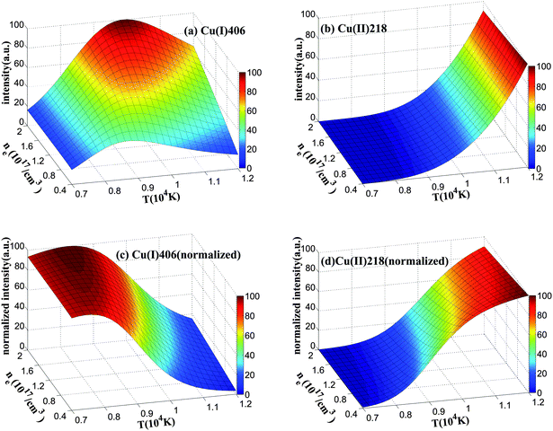Fig. 1 Change of calculated line intensity with plasma temperature and electron density. Two copper lines, Cu(I) 406 (left) and Cu(II) 218 (right), are studied. Here, (a) and (b) show the intensity without any normalization, while (c) and (d) show the intensity after normalization.

Table 1 The Cu emission lines selected for the segmental area normalization

Atomic line Cu(I)/nm	216.510, 261.837, 309.993, 310.860, 312.611, 327.396, 348.376, 402.263, 406.264, 427.511, 453.078, 529.252, 570.024, 578.213
Ionic line Cu(II)/nm	204.3802, 205.442, 214.898, 217.941, 224.262, 224.700, 226.379, 227.626, 229.437, 236.989, 250.627, 254.481

---

It can be observed from Fig. 1(c) and 1(d) that the trends of the intensity changes of the two lines with temperature are completely opposite. Hence, a combined intensity of an atomic and an ionic line is proposed:

I = cI^I_ij + (1 − c)I^II_mn, (5)

where c is the combination coefficient with a value between 0 and 1.

In this newly defined combined intensity, its components I^I_ij and I^II_mn are functions of T, α, and n_s. Here, n_e is regarded as dependent on T and α. The derivative of the intensities, dI^I_ij and dI^II_mn may be expressed as:

and

Using eqn (1) and (2), one may generate:

and

By setting a condition:

ca₂ + (1 − c)b₂ = 0, (10)

the derivative of I may be independent on the change of ionization degree α:

dI = cdI^I_ij + (1 − c)dI^II_mn = [ca₁ + (1 − c)b₁]dT + [ca₃ + (1 − c)b₃]dn_s. (11)

The combination coefficient, c, may be determined from eqn (10). Assume E^I_i ≈ E^II_m and the partition function U^I(T) and U^II(T) are insensitive to T,³¹ then the combination coefficient is a constant. As already shown by the change of plot's shape from Fig. 1(a)–(d), the effect of dn_s can be minimized by normalization. This leaves the combined intensity a function of T only.

Fig. 2 illustrates the change of the combined intensity (Cu(I) 406 nm and Cu(II) 218 nm) with T and n_e. The combination coefficient c is 0.72. In addition, the combination coefficient of this calculation was estimated through rough calculation by varying the combination coefficient until the surface in Fig. 2 looks rather flat. The simulation result indicates that the combined intensity is almost insensitive to the variation of plasma temperature or electron density within the range of interest. The signal has less fluctuation and the calibration model built by this data is supposed to be more robust and accurate.

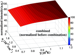Fig. 2 Change of the combined intensity (Cu(I) 406 nm and Cu(II) 218 nm) with n_e and T. The spectral lines are normalized before being combined. The combination coefficient is 0.72.

It should be noted that although the combination coefficient may be calculated from eqn (10), the assumptions of E and U(T) do not always hold for all combinations. Also, the line intensity can be modified by many factors such as self-absorption, line broadening, gate width of the spectrometer, or spectral response of the sensors. Therefore, a more practical approach is to adjust the coefficient c directly so that the average relative standard deviation (RSD) of the combined line across all calibration samples is minimized (see next section).

3 Experimental

The LIBS system used in this study was Spectrolaser 4000 which has been described in detail in a previous paper.²⁴Fig. 3 shows the schematic diagram of the system. The laser source was a Nd:YAG laser operating at its second harmonic. The energy was set at 90 mJ, and the pulse was focused by a 50 mm lens onto the target. The plasma emission was projected to four optical fibers by four collimators and transmitted to the detection system. The detectors were composed of four Czerny-Turner spectrographs, each equipped with a CCD sensor. Four spectrometers cover the wavelength range of 190–310 nm, 310–560 nm, 560–770 nm, and 770–950 nm, respectively. The gate delay was adjusted to 2.25 μs, and the integration time was 1 ms, which cannot be changed. The experiment was conducted under atmospheric environment.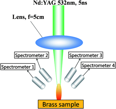

Fig. 3 Schematic diagram of the LIBS system.

The 29 brass alloy samples were supplied by Central Iron and Steel Research Institute (CISRI) of China and Shenyang Nonferrous Metals Processing Factory. Their major composition was Cu, Zn, Pb, and Fe. Copper was the element of interest, and its concentration was distributed from 56% to 97% (Table 2). Twenty samples were selected for calibration, while the rest were for validation. The samples for validation were chosen with their Cu concentration spread evenly across the available range. All samples were cleaned by anhydrous ethanol and left air-dried.

Table 2 29 brass samples for calibration and validation. Concentrations are in percentage weight. Numbers marked with * are validation samples

Sample	Cu (wt%)	Sample	Cu (wt%)
1	73	16*	95.1
2	60.28	17	94.46
3*	64.43	18	92.7
4	59.14	19	89.97
5*	58.07	20*	90.76
6	56.62	21*	85.49
7	59.55	22*	79.1
8*	59.89	23	70.44
9*	61.88	24*	69.25
10	69.08	25	67.59
11	80.9	26	64.32
12	85.06	27	63.42
13	90.02	28	60.81
14	95.9	29	57.98
15	96.86

---

Before the measurement, a cleaning shot of 150 mJ was fired at the sample surface to remove any contaminant. The same spot was then probed by a 90 mJ pulse. To avoid the crater effect, only one spectrum was collected from a position. A total of 35 positions were sampled and all spectra were background-subtracted before processing.

With 14 atomic and 12 ionic lines, a total of 168 combinations were generated to test the proposed combined line algorithm. Since there were four spectrometers used in our application, each emission line was normalized by the sum intensity of its own spectral area (so-called segmental normalization²¹) before being combined mainly to reduce the line intensity fluctuation due to total number density variation.

Since there are 35 laser shots on different locations on each sample, for each pair of atomic and ionic lines, the combined intensity was calculated for each of the 35 spots. Then the average value and RSD was calculated from the 35 combined intensities. For each pair of atomic and ionic lines, the combination coefficient was calculated by a recursive procedure, by varying the combination coefficient in the range of 0–1 until a minimized average RSD of the 20 calibration samples was obtained.

4 Results and discussion

Since the proposed method is based on the LTE condition, the LTE had been investigated, and results showed the McWhirter Criteria are satisfied for all samples and laser shots, so the relaxation time and diffusion length had been calculated according to ref. 33. The average relaxation time is about 5.3 μs and the average diffusion length is about 18 μm, with no big differences among different samples and laser shots. Since the relaxation time and diffusion length are much shorter than the plasma lifetime and size, we can believe that the plasma is in LTE condition.

Although our method is based on the LTE assumption, the method may be applied on non-LTE conditions as well, since the opposite change of the intensity of atomic lines and ionic lines is likely still kept for non-LTE condition. Of course, more experiments and investigations are required to verify this conclusion.

4.1 Uncertainty reduction

The stability of the combined signal is first evaluated by comparing its RSD with those of its composing lines. To quantify the comparison, an average RSD across the calibration set is first obtained for each combination. Then, a relative improvement of RSD for each combination can be defined as:

In general, all data points show an improvement in RSD when the combined intensity method is applied (Fig. 4(a)). Of 168 data points, 123 of RSD are improved by more than 10%. 40% of the RSD are even improved by more than 20%. The results confirm the effectiveness of the proposed model in reducing data fluctuation. It should also be noted that, although the combination coefficients are determined from the data of the calibration set, they also perform well with the validation set (Fig. 4(b)).

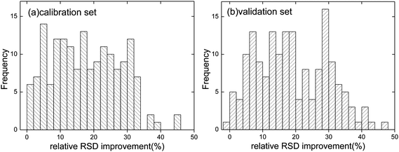Fig. 4 Distribution of the relative RSD improvement of the combined intensities of (a) the calibration set and (b) the validation set.

For simplicity, the pair which generates the lowest average RSD is chosen for further discussion. This pair is formed by Cu(I) 406 and Cu(II) 218 with a combination coefficient of 0.48. Among all selected lines, the best results (RSD, RMSEP, etc.) are obtained from Cu(II) 218 line if only single line analysis is considered. Therefore, in the following comparison, the combined line and the Cu(II) 218 line are focused.

Fig. 5 shows the RSD of the intensities of Cu(I) 406, Cu(II) 218, and their combined signal. The average RSD for all 29 samples is reduced from 2.93% (Cu(I) 406) and 2.13% (Cu(II) 218) to 1.68%. Clearly, the stability of combined line intensity is greatly improved when compared with its atomic and ionic counterparts.

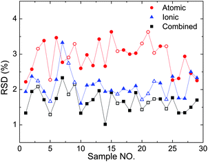Fig. 5 Comparison of the RSD of the atomic line intensity Cu(I) 406, ionic line intensity Cu(II) 218, and their combination intensity. The combination coefficient is optimized to be 0.48. The full symbols represent the calibration samples while the empty symbols represent the validation samples.

4.2 Accuracy improvement

A conventional univariate model can be constructed by correlating the copper concentration to the copper line intensity. Through combining the atomic line and ionic line, not only the uncertainty is reduced, but also the accuracy of concentration prediction may be improved. A standard calibration curve is first established by the calibration set. The concentration of a probed spot of a validation sample may then be retrieved from the plot. An average concentration and a standard deviation (SD) are calculated from the 35 sampling spots for each sample.

Fig. 6 shows the calibration curve for the atomic line Cu(I) 406, ionic line Cu(II) 218, and the combined signal. The open symbols represent the validation data. According to the plot, the coefficient of determination, R², is improved from 0.97 to 0.99. The error bars are also smaller in the combined signal data. Both observations indicate that a more robust model is established. For the validation, the root mean square error of prediction (RMSEP) decreases from 2.24% for Cu(I) 406 and 2.43% for Cu(II) 218 to 1.40% for the combined line. This is due to improvement of the data quality which increases the accuracy of the model.

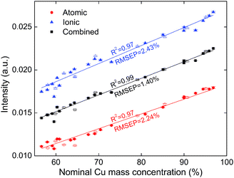Fig. 6 Calibration curves of copper concentration established from the atomic line intensity, ionic line intensity, and combined signal. The full symbols represent the calibration samples while the empty symbols represent the validation samples.

In practical applications, sometimes a single shot measurement is only allowed. Thus, the performance of single shot analysis should also be evaluated. A maximum relative error (MRE) is defined as:

where C is the certified concentration, and C^pred_i is the predicted value of an i analysis. In an ideal situation where the signal uncertainty is minimal, the MRE should also be the lowest.

The MRE are reduced when the combined signal is considered (Fig. 7), decreasing from 9.27% for Cu(I) 406, and 9.53% for Cu(II) 218, to 6.25% for combined intensity. Some samples even show a decrease of more than two-folds when compared to the worse MRE of the single line. Obviously, through combining the lines, the data quality for single shot analysis can be greatly improved.

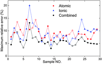Fig. 7 Maximum relative errors of atomic line intensity (Cu(I) 406), ionic line intensity (Cu(II) 218), and the combined signal. The full symbols represent the calibration samples while the empty symbols represent the validation samples.

Table 3 summarizes the performances of the Cu(I) 406, Cu(II) 218, and the combined signal. Overall, the combined signal algorithm generates the best results. The RSD and RMSEP significantly enhances when compared to the conventional single line method. The results suggest that the new signal is more stable with the change of the plasma temperature and electron density, which allows the construction of a better calibration model for a more accurate prediction. The improvement of the MRE also facilitates LIBS applications in which single shot measurement is necessary.

Table 3 Summary of results

	Cu(I) 406	Cu(II) 218	Combined
R ^2	0.97	0.97	0.99
Average RSD of the calibration samples (%)	2.85	2.18	1.68
Average RSD of the validation samples (%)	3.11	2.03	1.69
RMSEP (%)	2.24	2.43	1.40
MRE (%)	9.27	9.53	6.25

---

5 Conclusions

By utilizing the emission characteristics of an atom and an ion under different plasma temperatures and electron densities, a method combining the intensities of an atomic and an ionic line is proposed. The effect of the ionization degree may be minimized by a suitable choice of a combination coefficient. Using brass alloys as samples, the RSD is found to be greatly reduced and the R² is increased. This improvement helps to construct a more accurate model for concentration prediction which also performs well in single-shot analysis.

However, the proposed method requires ionic lines, so implementing to non-metal elements is challenging because these elements usually have a high ionization. Current work is focused on the application of the present method to non-metals in order to improve the measurement stability.

Acknowledgements

The authors are grateful for the financial support from the National Natural Science Foundation of China (no. 51276100).

References

1. J. D. Winefordner, I. B. Gornushkin, T. Correll, E. Gibb, B. W. Smith and N. Omenetto, J. Anal. At. Spectrom., 2004, 19, 1061–1083,  10.1039/B400355C.
2. L. J. Radziemski, Spectrochim. Acta, Part B, 2002, 57, 1109–1113,  DOI:10.1016/S0584-8547(02)00052-6.
3. D. A. Rusak, B. C. Castle, B. W. Smith and J. D. Winefordner, Crit. Rev. Anal. Chem., 1997, 27, 257–290,  DOI:10.1080/10408349708050587.
4. A. W. Miziolek, V. Palleschi and I. Schechter, Laser-Induced Breakdown Spectroscopy (LIBS): Fundamentals and Applications, Cambridge University Press, 2006.
5. R. E. Russo, X. Mao, H. Liu, J. Gonzalez and S. S. Mao, Talanta, 2002, 57, 425–451,  DOI:10.1016/S0039-9140(02)00053-X.
6. C. Sanchez-Ake, M. Bolanos and C. Z. Ramirez, Spectrochim. Acta, Part B, 2009, 64, 857–862,  DOI:10.1016/j.sab.2009.07.001.
7. A. M. Popov, F. Colao and R. Fantoni, J. Anal. At. Spectrom., 2009, 24, 602–604,  10.1039/B818849A.
8. J. M. Vadillo, J. M. F. Romero, C. Rodriguez and J. J. Laserna, Surf. Interface Anal., 1999, 27, 1009–1015,  DOI:10.1002/(SICI)1096-9918(199911)27:11<1009::AID-SIA670>3.0.CO;2-2.
9. A. Effenberger and J. Scott, Sensors, 2010, 10, 4907–4925,  DOI:10.3390/s100504907.
10. V. I. Babushok, F. C. DeLucia Jr, J. L. Gottfried, C. A. Munson and A. W. Miziolek, Spectrochim. Acta, Part B, 2006, 61, 999–1014,  DOI:10.1016/j.sab.2006.09.003.
11. X. Zeng, X. Mao, S. S. Mao, S.-B. Wen, R. Greif and R. E. Russo, Appl. Phys. Lett., 2006, 88, 061502–061503,  DOI:10.1063/1.2172738.
12. M. Pardede, T. J. Lie, K. H. Kurniawan, H. Niki, K. Fukumoto, T. Maruyama, K. Kagawa and M. O. Tjia, J. Appl. Phys., 2009, 106, 063303–063306,  DOI:10.1063/1.3224864.
13. G. W. Rieger, M. Taschuk, Y. Y. Tsui and R. Fedosejevs, Spectrochim. Acta, Part B, 2003, 58, 497–510,  DOI:10.1016/s0584-8547(03)00014-4.
14. A. E. Pichahchy, D. A. Cremers and M. J. Ferris, Spectrochim. Acta, Part B, 1997, 52, 25–39,  DOI:10.1016/s0584-8547(96)01575-3.
15. H. Kurniawan, M. M. Suliyanti, T. J. Lie, K. Kagawa and M. O. Tjia, Spectrochim. Acta, Part B, 2001, 56, 1407–1417,  DOI:10.1016/S0584-8547(01)00253-1.
16. D. Body and B. L. Chadwick, Spectrochim. Acta, Part B, 2001, 56, 725–736,  DOI:10.1016/S0584-8547(01)00186-0.
17. S. Y. Oh, F. Y. Yueh, J. P. Singh, C. C. Herman and K. Zeigler, Spectrochim. Acta, Part B, 2009, 64, 113–118,  DOI:10.1016/j.sab.2008.10.023.
18. F. Bredice, H. Sobral, M. Villagran-Muniz, H. O. Di Rocco, G. Cristoforetti, S. Legnaioli, V. Palleschi, A. Salvetti and E. Tognoni, Spectrochim. Acta, Part B, 2007, 62, 836–840,  DOI:10.1016/j.sab.2007.06.011.
19. Z. Wang, J. Feng, L. Li, W. Ni and Z. Li, J. Anal. At. Spectrom., 2011, 26, 2289–2299,  10.1039/c1ja10041f.
20. L. Fornarini, F. Colao, R. Fantoni, V. Lazic and V. Spizzicchino, Spectrochim. Acta, Part B, 2005, 60, 1186–1201,  DOI:10.1016/j.sab.2005.06.008.
21. J. Feng, Z. Wang, L. West, Z. Li and W. D. Ni, Anal. Bioanal. Chem., 2011, 400, 3261–3271,  DOI:10.1007/s00216-011-4865-y.
22. L. Xu, V. Bulatov, V. V. Gridin and I. Schechter, Anal. Chem., 1997, 69, 2103–2108,  DOI:10.1021/ac970006f.
23. U. Panne, C. Haisch, M. Clara and R. Niessner, Spectrochim. Acta, Part B, 1998, 53, 1957–1968,  DOI:10.1016/S0584-8547(98)00239-0.
24. J. Feng, Z. Wang, Z. Li and W. Ni, Spectrochim. Acta, Part B, 2010, 65, 549–556,  DOI:10.1016/j.sab.2010.05.004.
25. L. Li, Z. Wang, T. Yuan, Z. Hou, Z. Li and W. Ni, J. Anal. At. Spectrom., 2011, 26, 2274–2280,  10.1039/c1ja10194c.
26. L. Sun and H. Yu, Spectrochim. Acta, Part B, 2009, 64, 278–287,  DOI:10.1016/j.sab.2009.02.010.
27. J. B. Ahmed and N. Jaïdane, Spectrochim. Acta, Part B, 2009, 64, 442–447,  DOI:10.1016/j.sab.2009.04.011.
28. R. Mavrodineanu, Flame Spectroscopy, John Wiley & Sons, New York, 1965.
29. Plasma Spectroscopy, ed. H. R. Griem, McGraw-Hill Inc., New York, 1964.
30. Z. Chen and A. Bogaerts, J. Appl. Phys., 2005, 97, 063305–063312,  DOI:10.1063/1.1863419.
31. NIST, NIST Atomic Spectra Database, http://www.nist.gov/pml/data/asd.cfm, 2011.
32. Z. Wang, J. Feng, L. Li, W. Ni and Z. Li, J. Anal. At. Spectrom., 2011, 26, 2175–2182,  10.1039/c1ja10113g.
33. G. Cristoforetti, A. De Giacomo, M. Dell'Aglio, S. Legnaioli, E. Tognoni, V. Palleschi and N. Omenetto, Spectrochim. Acta, Part B, 2010, 65, 86–95,  DOI:10.1016/j.sab.2009.11.005.

---